A Hadoop ecosystem consists of the core application HDFS and peripheral applications, including Hive, HBase, Spark, and others. Hive is the easiest to access by the reporting tool because it provides official JDBC driver. Other applications are much more difficult to access because they offer API interface only. Most reporting tools can only invoke the API interface using a user-defined data set, and the code is extremely complicated. A few encapsulate API interface to make data retrieval simple, but the computing process is complex still and a lot of hardcoding work is needed.

A better choice is the open-source, Java-based class library SPL. SPL encapsulates the API interface as a simple and easy-to-use retrieval function that has uniform syntax, making it convenient to access both HDFS and a lot of peripheral applications. It has great computational capabilities and the JDBC driver is easy to be integrated by the reporting tool.

SPL offers convenient and easy-to-use retrieval functions that can retrieve data from various Hadoop data sources. For instance, HDSF stores structured files of many types and we are trying to retrieve data from them:

SPL can also retrieve data from files with non-standard formats and from multilevel JSON or XML.

Retrieve data from HBase:

Retrieve data from Spark:

Hive supplies both JDBC and API interfaces. The latter is higher in performance. SPL supports JDBC interface and encapsulates API interface. Their uses are as follows:

SPL has a wealth of built-in functions so that it can retrieve data using simple and intuitive syntax, without the need of any complicated hardcoding. To perform a query on orders data according to interval-style conditions, for instance, we have the following SPL code, where p_start and p_end are parameters:

SPL data retrieval processes are highly similar, and SPL syntax is universally applied. So, no detail will be explained separately about them.

As code written in an RDB, SPL code can be integrated into a reporting tool through its JDBC driver. Take the above SPL code as an example, we can first save it as a script file and then invoke its name in the reporting tool as we do with a stored procedure. Assume we are using Birt and the code can be like this:

{call intervalQuery(? , ?)}

More examples:

SPL also supports standard SQL syntax in order to help beginners adapt. The syntax is suitable for handling computing scenarios involving short and simple code. The above query based on interval-style conditions can be rewritten as the following SQL statement:

More examples can be found in Examples of SQL Queries on Files.

SPL’s most prominent feature is its outstanding computational capabilities, which simplify computations with complex logic, including stepwise computations, order-based computations and post-grouping computations. SPL can deal with many computations that are hard to handle in SQL effortlessly. Here is an example. We are trying to find the first n big customers whose sales amount occupies at least half of the total and sort them by amount in descending order.

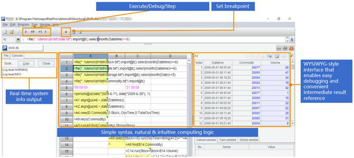
SPL has a professional IDE equipped with all-around debugging functionalities and letting users to observe the result of each step with grid-style coding, making it particularly suited to implementing algorithms with complex logic.

SPL also supports many more data sources, including WebService, RESTful, MongoDB, Redis, ElasticSearch, SalesForce, Cassandra and Kafka, and the mixed computations between any types of data sources or databases.