1.4 General data table operations
1.4.1 T function and E function
When using the import()/xlsimport function, it needs to define the file object first. Since the operation for reading and writing of the structured files is very common, SPL provides a simpler T() function, which can automatically take different actions based on the file extension.
| A | |
|---|---|
| 1 | =T(“data.txt”) |
| 2 | =T(“data.csv”) |
| 3 | =T(“data.txt”;”|”) |
| 4 | =T@b(“data.csv”) |
| 5 | =T(“data.xls”) |
| 6 | =T(“data.xlsx”) |
| 7 | =T(“data.xlsx”;“sheet2”) |
| 8 | =T@b(“data.xlsx”) |
A1: With title, columns to be separated by TAB
A2: With title, columns to be separated by comma
A3: With title, columns to be separated by |
A4: Without title, separated by comma
A5: With title
A6: With title
A7: With title, specify sheet
A8: Without title
T() function has also other parameters, which allow you to choose to read partial columns, and support writing. Because it is not very common, no examples are given here.
The data in Excel table often appears in the form of two-dimensional sequence, and it will be more convenient to convert the sequence to a table sequence when processing. SPL provides a short E function to process the said conversion:
| A | |
|---|---|
| 1 | =file(“data.xlsx”).xlsimport@w() |
| 2 | =E(A1) |
| 3 | =E@b(A1) |
| 4 | =E(A2) |
| 5 | =E@b(A2) |
A1: Read the Excel as a 2D sequence
A2: Convert two-dimensional sequence to table sequence, the first row is the title
A3: Without title
A4: Convert the table sequence to two-dimensional sequence, the first row is the title
A5: Ignore the title
E() function has other options, which allow you to convert the table sequence and TAB/Enter separated strings to each other. You can refer the documents to do experiments by yourself.
1.4.2 Filtering
Filter out the row that meets the condition from the data table.
Example: We want to filter out the student scores of Class 10 from the student score table Students_scores.txt. The first row in the file is the column name, and the data starts from the second row, as shown in the figure below.

| A | |
|---|---|
| 1 | =T(“E:/txt/Students_scores.txt”).select(CLASS==10) |
A1: Read the data in the file and then select the rows of class 10. The T function will automatically select the appropriate separator based on the file extension.
1.4.3 Summary
Summarize the data in the data table.
Example: Calculate the average score in Chinese, the highest score in math, and the total score in English for all students in the student score table.
| A | |
|---|---|
| 1 | =T(“E:/txt/Students_scores.txt”) |
| 2 | =A1.avg(Chinese) |
| 3 | =A1.max(Math) |
| 4 | =A1.sum(English) |
A1: read the data in the file.
A2: calculate the average score in Chinese
A3: calculate the highest score in Math
A4: calculate the total score in English
1.4.4 Cross-column calculation
Perform cross-column calculation on the data in the data table.
Example: calculate the total score of each student in the student score table.
| A | |
|---|---|
| 1 | =T(“E:/txt/Students_scores.txt”) |
| 2 | =A1.derive(English+Chinese+Math:total_score) |
A1: read the data in the file.
A2: add a column total_score in A1, and the value of this new column is the sum of English, Chinese and Math columns
The results in A2 are as follows:

1.4.5 Sorting
Sort the data in ascending/descending order.
Example: sort the student score table in ascending order by class number, and in descending order by total score.
| A | |
|---|---|
| 1 | =T(“E:/txt/Students_scores.txt”) |
| 2 | =A1.sort(CLASS) |
| 3 | =A1.sort(CLASS,-Math) |
A1: read the data in the file.
A2: sort in ascending order by class number
A3: first sort in ascending order by class number, and then sort in descending order by math score within the class
1.4.6 Grouping and aggregating
Group and aggregate the data in the data table.
Example: query the lowest score in English, the highest score in Chinese and the total score in Math for each Class.
| A | |
|---|---|
| 1 | =T(“E:/txt/Students_scores.txt”) |
| 2 | =A1.groups(CLASS;min(English),max(Chinese),sum(Math)) |
A1: read the data in the file.
A2: group by class, and calculate the lowest score in English, highest score in Chinese, and total score in math for each class.
1.4.7 Filter after grouping
Filter the data after they are grouped and aggregated.
Example: find the classes with an average English score below 70.
| A | |
|---|---|
| 1 | =T(“E:/txt/Students_scores.txt”) |
| 2 | =A1.groups(CLASS;avg(English):avg_En) |
| 3 | =A2.select(avg_En<70) |
A1: read the data in the file.
A2: group by class, and calculate the average English score of each class and name the new column as avg_En
A3: select those with an average English score of below 70 from A2
The query results in A3 are as follows:

1.4.8 Association
- Perform the associative calculation on the data in two data tables.
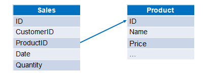
Example: The sales order information and product information are stored in two Excel files, respectively, and now we want to calculate the sales of each order. The data structure of the two files is as follows:

| A | |
|---|---|
| 1 | =T(“e:/orders/sales.xlsx”) |
| 2 | =T(“e:/orders/product.xlsx”).keys(ID) |
| 3 | =A1.join(ProductID,A2,Name,Price) |
| 4 | =A3.derive(Quantity*Price:amount) |
A1: read the sales order data.
A2: read the product information data, and set ID as the primary key
A3: associate A1 with the primary key in A2 according to the ProductID, and join the data of Name and Price columns at the same time
A4: add a column amount in A3, and its value is product of the sales Quantity and product Price
- Perform the associative query on the data in two data tables.
Example: We still use the above-mentioned two files to query the sales orders with product price greater than 20 dollars.
| A | |
|---|---|
| 1 | =T(“e:/orders/sales.xlsx”) |
| 2 | =T(“e:/orders/product.xlsx”).select(Price>20).keys(ID) |
| 3 | =A1.switch@i(ProductID,A2) |
A1: read the sales order data.
A2: read the product information data to select the product information with a price greater than 20, and then set the ID as the primary key.
A3: associate A1 with the primary key in A2 according to ProductID, the option @i means that when a product ID that matches the ProductID cannot be found in A2, this row will be deleted.
- Perform the associative query on the data in primary table and detail table.
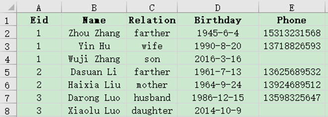
Example: Part of data in the employee information table (employee.xlsx) and employee family member table (family.xlsx) are as follows. Now we want to query the information of employees whose family has the elderly person over 70 years old.


| A | |
|---|---|
| 1 | =T(“e:/work/employee.xlsx”) |
| 2 | =T(“e:/work/family.xlsx”).select(age(Birthday)>=70) |
| 3 | =join(A1:employee,Eid;A2:family,Eid) |
| 4 | =A3.conj(employee) |
A1: read the employee information data
A2: read the employee family member data and select members over the age of 70
A3: associate A1 and A2 according to Eid, and filter to delete unmatched row, and name A1 as employee and A2 as family
A4: take out the employee column in A3 and concatenate as a table sequence
esProc Desktop and Excel Processing
1.3 Files and directories
2.1 Installation and Configuration
SPL Official Website 👉 https://www.scudata.com
SPL Feedback and Help 👉 https://www.reddit.com/r/esProc_Desktop/
SPL Learning Material 👉 https://c.scudata.com
Discord 👉 https://discord.gg/2bkGwqTj
Youtube 👉 https://www.youtube.com/@esProcDesktop
Linkedin Group 👉 https://www.linkedin.com/groups/14419406/


