Different from the traditional programming language, the application of set in SPL is very common. In fact, the most common sequence and sequence table are set in nature, and SPL can carry out real set operations on them, thus greatly improving the development efficiency and code performance. Therefore, when using SPL, we need to pay special attention to the understanding of set concept.

1 Sequence and set in SPL

In SPL, sequences, like integers and strings, are very common basic data types and can also perform corresponding basic operations. From the perspective of set, SPL provides the basic operators of set A and B: A^B, A|B, A&, A\B, etc. If we can start from these operations and use them skillfully, we can take the initiative to use set thinking when solving problems, so that we can make full use of the known data, the thinking is more direct and concise, and the method is simpler and clearer.

The following example shows how to use set operations to simplify code:

	A
1	=demo.query("select EID, NAME,   SURNAME, GENDER, STATE from EMPLOYEE")
2	=A1.select(GENDER=="M")
3	=A1.select(STATE=="California")
4	=A2^A3
5	=A1.select(GENDER=="M" &&   STATE=="California")
6	=A2&A3
7	=A1.select(GENDER=="M" ||   STATE=="California")
8	=A2\A3
9	=A1.select(GENDER=="M" &&   STATE!="California")

In the code, A4, A6 and A8 adopt set operation, and respectively count the male employees in California, all the males or the employees in California, and the male employees not in California. Compared with the traditional statistical methods of A5, A7 and A9, the form is significantly simpler.

However, it should be noted that although the employee data obtained in A6 and A7 are the same, the order recorded in the results is different, as follows:

 

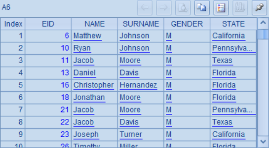
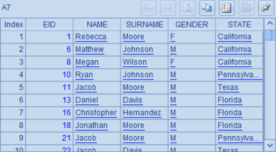
The reason for this is that the set in SPL is not exactly the same as the set in mathematics. The set in SPL is called an ordered set, which is ordered and can have duplicate members at the same time. Sequence, sequence table, array, etc. are all such ordered sets.

	A
1	[1,2,3,4]
2	[1,3,3,2]
3	=[1,2,3]==[1,3,2]

In the above table, the sequence in A2 has duplicate members, while the order of the members in the two sequences in A3 is different. When comparing them directly, they will be considered as unequal, and the result is false:

 

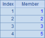
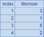
In addition, the intersection and union operations of sets in mathematics are commutative, i.e. a ∩ B º B ∩ A and a ∪ B º B ∪ A. However, since the sets in SPL are ordered sets, the exchange law does not hold. The result set of intersection and union operations will be subject to the order of left operands.

	A
1	[1,2,3]
2	[3,1,5]
3	=A1^A2
4	=A2^A1
5	=A1&A2
6	=A2&A1

 

The calculation results in A3, A4, A5 and A6 are as follows:

Because the sequence in SPL is an ordered set, the function A.eq(B) should be used to determine whether two sequences have the same members instead of the comparator ==:

	A
1	=[1,2,3]==[3,2,1]
2	=[1,2,3]==[3,2,1].sort()
3	=[1,2,3].eq([3,2,1])
4	=[1,2,3].eq([3,2,2])
5	=[1,2,2,3].eq([3,2,1,2])
6	=[1,2,2,3].eq([3,2,3,1])

A1 and A2 determine whether the two sequences are the same, and the results are as follows:

 

This is because when [3,2,1] in A2 performs sorting, the result is [1,2,3], and the order is the same as A1.

A3, A4, A5 and A6 all use the function A.eq(B) to determine whether the two sequences have the same members. The results are as follows:

 

If all members of two sequences are the same, they are called substitutable sequences. In particular, if there is a duplicate member in the sequence, the same number of duplicates is required for that member in its substitutable sequence.

2 Loop function

With the set data type, many operations on the members of the set can be written out in a single sentence easily, and there is no need to write loop code.

	A
1	[3,4,1,3,6]
2	=A1.sum()
3	=A1.avg()
4	=A1.max()-A1.min()

In the above table, four loop functions are used. Sum()in A2 is used to calculate the sum of the members in the sequence, avg() in A3 is used to calculate the average value of the members in the sequence, and max()and min() in A4 are used to calculate the difference between the maximum value and the minimum value in the sequence. Their calculation results are as follows:

 

When calculating a loop function, you can not only use the value of the set member itself, but also use the value calculated by the member, including the calculation result of the member value and the attribute value of the set member with structure. In this case, you can indicate the calculation formula in the parameter of the function, where the symbol ~ represents the current member in the loop calculation.

	A
1	[3,4,1,3,6]
2	=A1.sum(~*~)
3	=demo.query("select * from   EMPLOYEE")
4	=A3.min(~.BIRTHDAY)
5	=A3.min(BIRTHDAY)
6	=A3.avg(interval@y(BIRTHDAY,HIREDATE))

A2 in the above table calculates the sum of squares of the members in the sequence, that is, the square of each member value is accumulated circularly, and the result is as follows:

 

A4, A5, and A6 loop the attribute values of each member in the set generated by A3. A3 generates a set after querying the employee information sequence table, in which each member is an employee's information. In A4, the earliest birthday of an employee is calculated, that is, the minimum birthday of a member. The result is as follows:

 

The ~. in the A4 expression can be omitted and written as A5, so the calculation result is the same as A4.

In A6, calculate the average entry age of all employees, that is, the average value of the year difference between the time of entry and the time of birthday of each member. The result is as follows:

 

Executing aggregation functions with parameters can be understood as two steps:    

1)        First, each member of the set is computed according to the parameter expression, and the result is called the calculated column.          

2)        Aggregate calculation of calculated columns.

In form, it can be expressed as: A.f(x)=A.(x).f().For example, A1.sum(~*~) is equivalent to A1.(~*~).sum(), where A1.(~*~) is the calculated column function，that is, the square of each member in A1 is calculated and returned as a sequence. 

In the above example, A5 and A6 omit the symbol ~. This is because only one layer of loop function is used, omitting ~ will not cause ambiguity. If the nested loop function is used, ~ will be interpreted as a member of the inner sequence. In this case, if you want to reference the outer sequence member, you must add the outer sequence name before ~.

	A
1	[A,B,C]
2	[a,b,c]
3	=A1.(A2.(~/~))
4	=A1.(A2.(A1.~/~))
5	=A1.(A1.(A1.~/~))
6	=A1.((arg=~,A1.(arg/~)))

String concatenation / is used in this example. In A3, two letters are spliced in the loop using /, but ~ can only get the members of inner sequence A2, so the resulting string is only two repeated lowercase letters. While A4 indicates that the former ~ corresponds to the outer sequence during the loop, so the result is that A1 capital letter is spliced in the front and A2 lowercase letter in the end. In the expression of A5, even though the inner loop uses A1.~, it can't identify which layer of A1 it is, so it can't refer to the outer A1 member, so it can only use the members in the inner sequence when calculating, and the result is the repeated capital letters. In this case, if you need to reference the outer member, you need to use the method of A6, first assign the outer member value to the temporary variable, and then use the temporary variable reference, so you can get the result of cross splicing of capital letters. The calculation results in A3 ~ A6 are as follows:

 

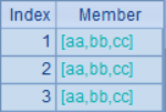
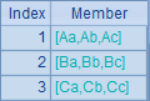
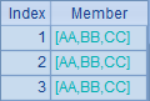
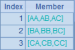
The rule about ~ is also applicable to the loop calculation of sequence table or array. If the field reference of ~ is omitted, the field will be interpreted as the field of inner array in priority. If the specified attribute field cannot be found in inner array, it will be found in outer layer.

 

3 Loop order

In short, the loop function will be calculated in the order of the original sequence, and we can make full use of this feature when we use it.

	A
1	[1,3,2,5,4,8,7]
2	0
3	=A1.(A2=A2+~)
4	[1,1,0,0,1,0,0,0,1,0,1,0,0,0]
5	0
6	=A4.max(if(~==0,A5=A5+1,A5=0))

In A3, the accumulated sum sequence of members in A1 is calculated by loop.

 

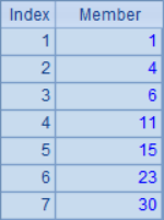
In A6, the longest number of consecutive members 0 in sequence A4 is calculated:

 

In many similar cases, we can write the effect equivalent to simple loop code with only one expression.

4 Sequence calculation

In addition to the above loop functions (such as sum, avg) that return a single aggregate value, we still need to continue to calculate the set in many cases. In addition to generating a new set with basic set union, intersection, minus and other operations, using the sequence calculation function A.(x) to return a set is also a very common method.

	A
1	[1,2,3]
2	=A1.(~*~)
3	=A1.(~)
4	=A1.()
5	=A1.(1)
6	=A1.(if(~%2==0,~,0))
7	I love you
8	=len(A7).(mid(A7,~,1))
9	=A8.count(~=="o")

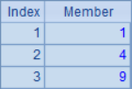
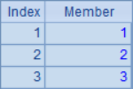
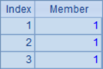
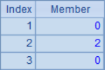
In the example, A2 ~ A6 generate different new sequences according to the calculation of sequence A1: A2 computes the square of each member; A3 and A4 generate new sequences with the members of the original sequence; A5 generates a sequence with the same number of members as the original sequence, but the members are all 1; A6 is slightly more complex, judge the members of A1 one by one in the loop calculation, if it is odd, get 0, otherwise get the corresponding  value of the member. The calculation results of A2 ~ A6 are as follows:

 

 

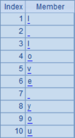
The complete writing of A8 is =to(len(A7)).(mid(A7,~,1))，where the to(n) function generates a new sequence of numbers from 1 to n (like the preceding symbol ~ , can be omitted in some cases). Loop this sequence, take out the strings in A7 one by one, so as to expand it into a sequence of single characters; A9 calculates the number of times the letter o appears in it. The results in A8 and A9 are as follows:

 

In addition to the return sequence, we can return the sequence table after calculating the sequence. We need to use the new function at this time.

	A
1	[1,2,3,4,5]
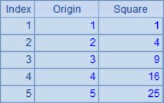
2	=A1.new(~:Origin,~*~:Square)
3	=demo.query("select * from   EMPLOYEE")
4	=A3.new(NAME,age(BIRTHDAY):Age)
5	=A3.new(NAME)
6	=A3.(NAME)

A2 returns a new sequence table based on A1 loop calculation, which contains two fields, one is the member in A1, and the other is the square value of the member. The ~ in the expression, which has been described before, represents the current sequence member in the loop. The result is as follows:

 

A3 takes the data from the data table employee to generate a sequence table. A4 obtains the name and birthday fields from the sequence table, calculates the age of the employee according to birthday, forms a new field age, and finally generates a new sequence table containing the name and age fields. The result is as follows: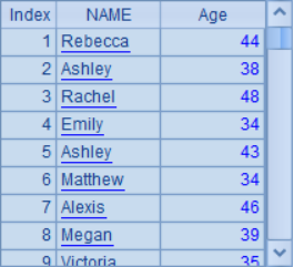 

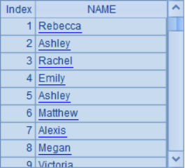
A5 and A6 look similar, but they are different in fact. A5 takes the name field from the A3 sequence table and directly generates a new sequence table containing a name field. A6 calculates the sequence composed of name field according to the A3 sequence table in loop. The difference between the two results is that the sequence table has data structure but the sequence has no data structure:  

In addition, there is a run function only used for calculation, which directly modifies the original sequence itself, rather than returning a new result sequence after the alignment calculation. Generally, it is used to modify the field value for the array (sequence table).

	A
1	=demo.query("select * from   EMPLOYEE")
2	=A1.new(NAME,age(BIRTHDAY):Age)
3	=A2.run(Age=Age+1)

In the example, a new sequence table is generated in A2, listing the names of employees and calculating their ages. In A3, the age of each employee is increased by 1. The run function changes the data in the original sequence table A2, so the results in A2 and A3 are the same, and the modified results will be returned together. Using step-by-step execution, you can see the change of sequence table in A2: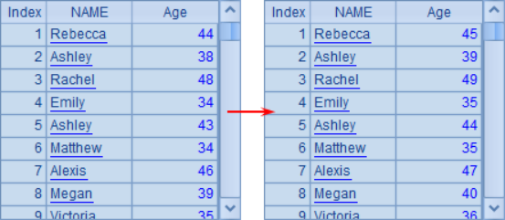

5 Genericity of sets

SPL does not require the data types of sequence members to be identical, so it is entirely possible to take values, strings, and complex records as members of the same sequence.

	A
1	[1,a3,2,5.4,$[4.5],2011-8-8]
2	=[A1,4]

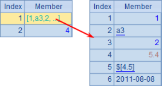
A1 contains members of various data types, while the sequence in A2 is composed of sequence A1 and an integer member. The data in A1 and A2 are as follows: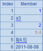 

 

For a general sequence, in most cases, it does not have much practical business significance to put different types of data in the same sequence, so it is not necessary to pay too much attention.

However, for permutations, that is, sequences composed of records, which are allowed to be composed of records from different sequence tables, it will be really convenient.

	A
1	=demo.query("select * from   EMPLOYEE")
2	=demo.query("select * from   FAMILY")
3	=A1|A2
4	=A3.count(left(GENDER,1)=="F")

A4 calculate the total number of women in the staff and family. Even if the structure of the employee table and the family table are different, as long as they contain the gender field, they can be calculated normally.

From this example, it can be seen that SPL does not care whether the records in the permutation come from the same sequence table. As long as they have fields with the same name, SPL can perform the same operation on them. This is far different from SQL, where you have to combine two tables with different structures into a new table by using the union statement. In this way, not only the thinking is clear and the writing is simple, but also the redundant memory will not be occupied, and the operation efficiency is higher.

6 Set of sets

In particular, the arbitrariness of set members also allows the set itself to be a member. At the same time, when A is a set of sets, you can further use the functions A.conj()，A.union()，A.diff()，A.isect() to calculate the sum column, union column, difference column and intersection column of each set in A.

 

	A
1	[[1,2,3,4,5],[1,3,5,7,9],[2,3,5,7]]
2	=A1.conj()
3	=A1.isect()
4	=A1.(~.sum())
5	=A1.(~.(~*~))

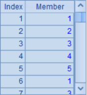
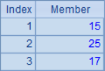
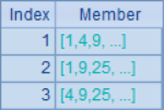
A1 is a sequence of sequences. A2, A3, A4 and A5 respectively calculate the sum sequence, intersection sequence, sum result of each sequence and the sequences composed of the square of each member of each sequence in A1. After calculation, the results in A2-A5 are as follows:

 

 

Similarly, an array can also be a member of a sequence.

	A
1	=demo.query("select EID, NAME,   SURNAME, GENDER, STATE from EMPLOYEE")
2	=A1.select(STATE=="California")
3	=A1.select(STATE=="Indiana")
4	=A1.select(STATE=="Florida")
5	=[A2,A3,A4]
6	=A5.(~.count())
7	=A5.(~(1).STATE)
8	=A5.(STATE)
9	=A5.new(STATE,~.count():Count)

In A2, A3 and A4, employee data of California, Indiana and Florida are extracted respectively. The sequence obtained in A5 is composed of three arrays A2-A4, which is a set of sets: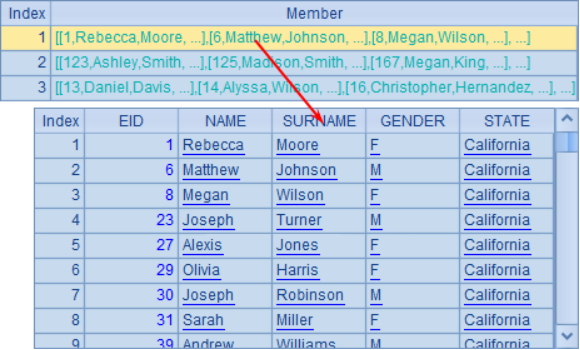

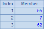
A6 calculate the number of employees in each state as follows:

 

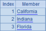
Take out the names of states in A7, and the ~(1) in the expression can be omitted, that is to say, A8 and A7 are equivalent, and the result is the same:

 

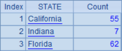
A9 has the same effect as A6, and it also counts the number of employees in three states. However, a new sequence table is generated through new, which is more clear and convenient for later retrieval according to the state name:

 

7 Understanding Grouping

Grouping is a very common operation in SQL, but not everyone can understand it deeply.            

From the perspective of set, the essence of grouping operation is to divide a set into several subsets according to some rules, that is to say, its return value should be a set composed of several sets. However, people often do not need to directly look at these subsets in the set, but are more interested in some aggregate values of subsets. Therefore, grouping is often accompanied by further aggregate calculation of subsets.

This is how SQL processes. Its group by statement always matches the corresponding aggregate calculation. Of course, this is also because SQL itself does not have an explicit set data type, so it cannot directly return data such as "set of sets". It can only force the aggregate calculation to the group calculation.

As time goes by, people get used to the fact that grouping always needs to cooperate with the subsequent aggregate calculation, and forget that grouping and aggregation are actually two independent steps.

 

But in any case, sometimes we are still interested in these grouping subsets. Moreover, even if you are only interested in the aggregate value, it is also valuable to keep these subsets, because if you can reuse them and don't have to regenerate them every time, it will be very helpful in code simplicity or performance improvement.

For SPL, because it fully realizes set thinking, it can restore the original meaning of grouping operation. In fact, the basic grouping function in SPL is only to do pure grouping, but to separate the aggregate calculation.

	A	B
1	=demo.query("select * from   EMPLOYEE")
2	=A1.group(month(BIRTHDAY),day(BIRTHDAY))	/Group employees by birthday (month, day)
3	=A2.select(~.len()>1)	/There are other employees with the same birthday
4	=A3.conj()
5	=A1.group(STATE)	/Group employees by state
6	=A5.new(~(1).STATE:State,~.count():Count)	/Use group results to calculate sequence table, number of employees in each state
7	=A5.new(STATE,~.avg(age(BIRTHDAY)):Age)	/ Calculation sequence table, average age of employees in each state

 

The result of grouping itself is a set of sets, so of course, you can continue grouping. Each member of the grouping result set is also a set, and each member can continue grouping. These are two different operations, but both form multi-level sets.

	A	B
1	=demo.query("select * from   EMPLOYEE")
2	=A1.group(year(BIRTHDAY))	/ Group by employee year of birth
3	=A2.group(int(year(~(1).BIRTHDAY)%100/10))
4	=A2.group(int(year(BIRTHDAY)%100/10))
5	=A2.(~.group(month(BIRTHDAY)))	/ Group the grouped results again, and A3, A4 and A5 will all return the sequence of arrays

If the level of set operation result is too deep, the real business meaning may not be very big, but it can be used to understand the thinking mode of set and the essence of operation. 

At the same time of grouping, the group function will sort all groups according to the result of grouping expression, such as:

	A	B
1	$ select EID,NAME+' '+SURNAME FULLNAME,   DEPT from EMPLOYEE
2	=A1.group(DEPT)	=A2.new(~.DEPT:DEPT,~.count():Count)
3	=A2.sort(~.DEPT:-1)	=A3.new(~.DEPT:DEPT,~.count():Count)
4	=A1.group@u(DEPT)	=A4.new(~.DEPT:DEPT,~.count():Count)
5	=A1.group@o(DEPT)	=A5.new(~.DEPT:DEPT,~.count():Count)

The sequence obtained in A1 is as follows:

 

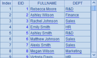
In A2, employee data is grouped by department name. By default, the grouping results in A2 are sorted in ascending order by department name. In column B, the number of people in each department under various grouping conditions is counted, so that the sorting can be viewed directly through the dept column. The results in A2 and B2 are as follows:

 

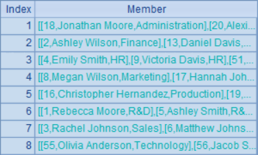
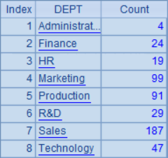
A3 changes the grouping results in A2 to sort by department descending order. The effect can be seen in B3. The results are as follows:

 

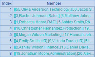
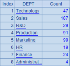
In addition to reordering the grouping results, you can also add options to adjust the grouping order when executing the group.            

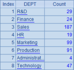
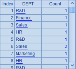
Add the @u option to A4 to keep the original order of departments in the employee table when grouping.

The @o option added in A5 specifies that the records will not be sorted as a whole when grouping, but only the adjacent records with the same grouping expression will be divided into a group, so it is more like "adjacent merge". Obviously, the "duplicate" grouping may occur in this situation. B4 and B5 show the effect of both:

 

8 Non-equi grouping

In addition to the regular group function, SPL also provides the A.align@a() function for handling aligned groups and A.enum() function for handling enumerated groups.

We call the grouping completed by group function equivalent grouping, which has the following characteristics:

1) any member of the original set must be in and can only be in a subset, that is, the grouped subset members completely cover the original set, and there is no overlap between the subsets;

2) no empty subsets 

But aligned grouping and enumeration grouping do not necessarily meet these two points.

Aligned grouping refers to the calculation of grouping expression with members in the set, and the completion of grouping according to the calculation result and the value in a sequence specified in advance. To align groups, you need to do the following:            

1) specify a set of values in advance            

2) divide a member in the set to be grouped whose calculation result is the same as the specified value into the same subset            

3) each subset of the result will correspond to the specified value one by one.

Under this grouping rule, there may be a member that is not in any subset, an empty set, or a member that exists in both subsets.

As the following example, employees are grouped in a specified state sequence:

	A
1	=demo.query("select * from   EMPLOYEE")
2	[California,Florida,Chicago]
3	=A1.align@a(A2,STATE)

In A3, set A1 is aligned and grouped according to A2, and the state name of A1 member corresponds to A2 member. In such a grouping process, some employees may not be in any group (employees in other states), or there may be an empty group without any members (Chicago is not a state name, and there is no corresponding employee at all). For example, in the case of some data, A3 results:

 

 

Enumerative grouping refers to specifying a set of conditions in advance, calculating the conditions by taking the members in the set to be grouped as parameters, and dividing those who satisfy the conditions into corresponding subsets. At this time, there may be a member that is not in any subset, or an empty set, or there may be members in two subsets at the same time.            

As the following example, group employees according to the specified age group:

	A
1	=demo.query("select EID, NAME,   SURNAME, GENDER, BIRTHDAY from EMPLOYEE")
2	[?<=35,? <=45,?>45]
3	=A1.enum(A2,age(BIRTHDAY))
4	[?<=35,?>20 && ?<=45,?>45]
5	=A1.enum@r(A4,age(BIRTHDAY))

In A3, the groups are enumerated according to the age condition sequence in A2. When the enum()function does not specify an option, the grouping result is not allowed to duplicate. That is to say, the record of an employee in A1 may not be in any group (but the conditions in the example are fully covered), but it will not appear in two groups at the same time (that is, it will not overlap). A3 result is as follows:

 

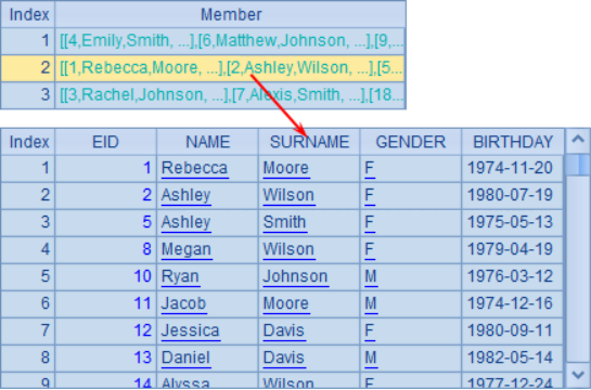
At this point, a young (under 35) employee is assigned to the first group. Since overlapping is not allowed, even if he meets the second condition, he will not be repeatedly assigned to the second group under the age of 45.

A5 also enumerates and groups according to the sequence of conditions in A4. However, @r option is added when enum function is used to indicate that grouping can be duplicated. At this time, the records of an employee may appear in multiple groups at the same time. For example:

 

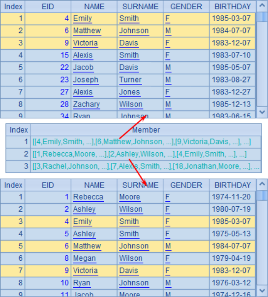
As you can see, some employee records exist in the first two groups at the same time. 

Although the align@ a function and enum function seem to be quite different from the group function, after understanding the essence of grouping operation, we can understand that they are all doing the same thing: that is, splitting a set into several subsets, the only difference is that the specific conditions and rules of splitting are different.