In the report data statistics, the data often needs to be rounded according to the requirements of precision or unit conversion, which is called rounding. Simple and direct rounding may bring hidden dangers, and the original balanced data relationship may be broken.

In order to ensure the correct data relationship in the report, it is necessary to adjust the data after rounding to make the data balance again. Such adjustment is called rounding balance. Here we will discuss how to use esProc to deal with the rounding balance problem.

Rounding calculation is often adopted in rounding processing, and errors will be generated. If there is a total value of these data in the report, the errors generated during rounding will accumulate, which may lead to the mismatch between the rounded data and its total value. For example, the original data with one decimal place is 4.5 + 4.5 = 9.0, and after rounding only the integer part, the balance relationship becomes 5 + 5 = 9, which seems obviously absurd. In this case, it is necessary to adjust the rounding result of non total data under the condition of keeping the total value correct, so as to rebalance the data relationship, for example, adjust to 4 + 5 = 9. This simple example is a typical rounding balance.

1. One way rounding balance

If each data is only used once for total value calculation in data statistics, then when processing rounding balance, you only need to adjust the used data according to the error of the total value, which is a relatively simple case. For example:

	A	B	C
1	[1.48,0,1.42,0.32,6.48,0.98,1.39]	=A1.sum()
2	=A1.(round(~))	=round(B1)	=A2.sum()

Some data are stored in the sequence of A1, and their total value is calculated in B1. The results are as follows:

 

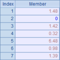
Now, round up the data to integers and make statistics again. In A2, each data in the sequence is rounded with round function to get a new sequence. In B2, the result in B1 is rounded, which is the result that should be obtained after data rounding. In C2, we simply use the data after rounding to sum. The results in A2, B2 and C2 are as follows:

 

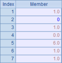
Obviously, the accumulation of error after rounding leads to the imbalance of data. After rounding the original data respectively, the total value changes from 12 to 10. So, can we change the total directly to 10? This is not possible because it will make the final result completely inconsistent with the real value. Therefore, in order to keep the balance after rounding, we should change the results after rounding each original data separately.            

The total error after rounding is called "balance difference". Rounding balance is actually the process of eliminating balance difference. There are many rules to deal with rounding balance. Let's study them separately:

(1) collate the balance difference into the first data. Namely:

	A	B	C
1	[1.48,0,1.42,0.32,6.48,0.98,1.39]	=A1.sum()
2	=A1.(round(~))	>A2(1)+=round(B1)-A2.sum()	=A2.sum()

In B2, the balance difference is converted to the first data after rounding. After finishing, the total value after rounding balance treatment is recalculated in C2. The results in A2 and C2 are as follows:

 

This rule of rounding balance is the simplest. However, after rounding, the first data changes from 1.48 to 3, which obviously deviates a lot. Therefore, such processing is not reasonable, especially in the case of a lot of data, the balance difference may also accumulate a lot, which leads to a very absurd migration result of the first data.

 (2) Share the balance difference according to the "minimum adjustment value" and adjust the data with large absolute value.            

The so-called minimum adjustment value is the unit value of the minimum precision after rounding. For example, when rounding to integers, the minimum adjustment value is 1 or - 1. If the total value becomes smaller after rounding, you need to increase the data, then the minimum adjustment value is 1; if the total value becomes larger after rounding, you need to decrease the data, and the minimum adjustment value is - 1. The adjustment is only for the data with larger absolute value, so their relative deviation will be smaller. The specific adjustment number is the total deviation divided by the minimum adjustment value.            

Under this rule, the rounding balance of the previous problem is handled as follows:

	A	B	C
1	[1.48,0,1.42,0.32,6.48,0.98,1.39]	=A1.sum()
2	=A1.(round(~))	=round(B1)-A2.sum()	=sign(B2)
3	=A1.psort@z(abs(~))	>abs(B2).run(A2(A3(#))+=C2)	=A2.sum()

Because it is only a rounding operation, the minimum adjustment value calculated in C2 is the positive or negative deviation of the total value;            

In A3, a sort is made according to the absolute value of the original data from large to small, and the result is the sequence number after sorting.            

B3 is the most important, because it is only a rounding to integer operation, so the number of original data to be adjusted is the absolute value of the deviation in B2. In this loop, the minimum adjustment value is allocated in turn according to the absolute value of the original value.            

C3 is the revalidation of the total value of the adjusted A2.

After adjustment, the results in A2 and C3 are as follows:

 

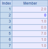
In this solution, the balance difference is shared by multiple data, and choosing the data with the largest absolute value will make the relative change of data minimum. Among the results, 1.48 rounding changed to 2, 6.48 rounding changed to 7, and the result of adjusting the balance was ideal.            

This solution needs to sort the data according to the absolute value, and the execution efficiency is not very good, especially in the case of large amount of data, sorting will take a lot of time.

(3) According to the minimum adjustment value, the balance difference is shared by the data that is not 0 in turn.

In the previous solution of adjusting rounding balance, the error is shared by the data with the largest absolute value. In practice, in order to improve the efficiency and reduce the sorting operation, we can simplify it properly and share the balance among data in the first few places. Considering that 0 does not produce error when rounding, and if 0 in the data is modified, such change will be more obvious, so 0 in the original data will remain unchanged when adjusting.

Under this rule, the rounding balance of the previous problem is handled as follows:

	A	B	C
1	[1.48,0,1.42,0.32,6.48,0.98,1.39]	=A1.sum()
2	=A1.(round(~))	=round(B1)-A2.sum()	=sign(B2)
3	=A2.pselect@a(~!=0)	>abs(B2).run(A2(A3(#))+=C2)	=A2.sum()

A3 selects the sequence number of the non 0 members in the original data, and then shares the adjustment in turn in B3 when adjusting the data. After adjustment, the results in A2 and C3 are as follows:

 

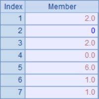
In the results, 1.48 rounding changed to 2, 1.42 rounding changed to 2, the result of adjusting the balance is more reasonable. At the same time, this solution avoids sorting operation and has high efficiency, so this rounding balance rule is most commonly used.

 

When dealing with one-way rounding balance, it is not only to sum a set of sequences. In more cases, it is to sum a batch of data, such as the sequence table stored in salesrecord.txt below:

 

Name      Jan  Feb  Mar Apr Allen      26106     49637     27760     33829 Billy       56611      50588     54765     76072 Charlie    21249     96825     28645     55958 Daisy      3413       49069     6279      98247 Flora       7590       12072     90034     64252

 

Now, you need to count the total sales of each employee for 4 months, which is in thousands of yuan, and handle rounding balance. The code is as follows:

	A	B	C	D
1	=file("SalesRecord.txt").i mport@t()	=A1.derive(Jan+Feb+Mar +Apr:Sum)	=B1.derive()
2	>5.(C1.field(#+1,C1.field(# +1).(round(~/1000))))	=C1.derive(Jan+Feb+Mar +Apr:Sum2)
3	for B2	>func(A5,A3)
4	=B2.derive(Jan+Feb+Mar +Apr:Sum3)
5	func	=A5.Sum-A5.Sum2	=abs(B5)	=sign(B5)*1
6		for C5	=A5.field(1+B6)	>A5.field(1+B6,C6+D5)

Execute the code step by step. After reading the sequence table in A1, add the sum field in B1. The result is as follows:

 

Copy the above sequence table in C1, and perform rounding calculation on the second to sixth fields in B1 to thousands. At this time, it is possible to break the balance due to rounding calculation, and add another field sum2 in B2 to calculate the total value of 4 months after rounding. The sequence table in B2 is as follows:

 

You can see that at this time, sum and sum2 fields are different, indicating that rounding balance needs to be adjusted. Although the data in the calculated sequence table needs to be adjusted here, each data is only used to calculate employee totals, so it still belongs to one-way rounding balance.

The subroutine in A5 is used to process the rounding balance of one piece of record. The balance difference is calculated in B5 and the minimum adjustment value is calculated in C5. In B6, the balance difference is split into the first few data in the record. Here, it is simply processed, without judging whether the data is non-zero.

In A3, the records in the sequence table B2 are looped and respectively adjusted for rounding balance. After adjustment, add sum3 field in A4 to verify rounding balance result. The result in A4 is as follows:

 

Comparing sum with sum3, it can be confirmed that the result is adjusted and the data is rounded to reach a balance again.

2. Bidirectional rounding balance

If the total value of data needs to be calculated in both row and column directions, and the total value of all data needs to be calculated at the same time, it is much more complicated to process rounding balance in this case. When processing rounding balance, not only the final total value is required to be accurate, but also the total value calculated in row and column directions is balanced with the data of corresponding rows and columns. In this case, rounding balance is called bidirectional rounding balance. For example, in the data of salesrecord.txt, you need to count the total sales of each month. The code is as follows:

	A	B	C
1	=file("SalesRecord.txt").import@t()	>A1.insert(0,"Total")	>4.(A1.m(-1).field(#+1,A1.field(#+1).to(,   5).sum()))
2	=A1.derive(Jan+Feb+Mar+Apr:Sum)	=A2.derive()	>5.(B2.field(#+1,B2.field(#+1).(round(~/1000))))
3	=B2.derive(Jan+Feb+Mar+Apr:Sum2)	=A3.derive(Sum2-Sum:Diff)	>B3.insert(0,"Total2")
4	>5.(B3.m(-1).field(#+1, A3.field(#+1).to(,5).sum()))	>B3.insert(0,"Diff")	>5.(B3.m(-1).field(#+1,B3(6).field(#+1)-   B3(7).field(#+1)))

Read in the sequence table in A1, and add a record in B1 to calculate the total sales of each month in D1. Then add a field in A2 to calculate the total sales amount of each employee and the total value. The result is as follows:

 

In C2, according to the above summary data, round the result to thousands. Then, according to the data after rounding, add the field sum2 in A3 to calculate the total employee value after rounding, and add the field diff in B3 to record balance difference of the employee total. Finally, two more records are added to calculate the total rounding value of each month and the balance difference. After calculation, the results in B3 are as follows:

 

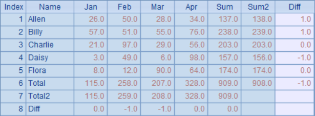
It can be seen that the balance problem to be solved after rounding is much more complicated when summarizing horizontally and vertically respectively. In this case, modifying any rounding data will affect the total calculation in both horizontal and vertical directions. Such a problem is called bidirectional rounding balance. In the above calculation, some balance differences are only related to the total value. For example, the balance difference on the far right side of the total row is only related to the total of each month. Such balance difference is called the aggregate balance difference. In the bidirectional rounding balance table, there is only one horizontal and one vertical aggregate balance difference. Other balance differences will be related to specific data, such as the lowest balance difference of Feb, which is called none aggregate balance difference.

 

We start with some simple cases to study the bidirectional rounding balance:            

(1) The symbol of none aggregate balance difference in horizontal and vertical direction is the same. As follows:

1.44	1.35	2.79
1.2	0	1.2
2.64	1.35	3.99

In the above table, the initial data of 2 rows and 2 columns are stored, and the total value of each row and column, as well as the total value of all data are calculated. These data are rounded to the nearest whole and the balance difference of each row / column is calculated as follows:

1	1	3	+1
1	0	1
3	1	4
+1

The "non aggregate balance difference" here refers to the balance difference involving the original data. At this time, neither the total data nor the total value needs to be adjusted. It can be seen that at this time, only the total value of row 1 and column 1 is unbalanced, and the total value is greater than the sum of rounding data by 1. In this case, only the data at the intersection needs to be adjusted, and the minimum adjustment value can be added or subtracted according to the balance difference symbol. The specific operation is to round the data at the intersection, i.e. row 1, column 1, to + 1 to get the balance. The results are as follows:

2	1	3
1	0	1
3	1	4

 

(2) In the same direction, the two signs of none aggregate balance difference are opposite. As follows:

1.44	1.55	2.99
1.2	0.85	2.05
2.64	2.4	5.04

Round these data and calculate the balance difference of each row / column as follows:

1	2	3
1	1	2
3	2	5
+1	-1

In this case, there is still no need to adjust the total value. As the balance difference in column 1 and column 2 is positive and negative respectively, only one row of data with balance difference of 0 needs to be selected, and the number of these two columns is added and subtracted by the minimum adjustment value according to the sign of balance difference. If the first row is selected, the rounding result of the first column + 1 and the rounding result of the second column - 1 will be balanced. The results are as follows:

2	1	3
1	1	2
3	2	5

 

(3) The sign of an aggregate balance difference is opposite to the sign of a none aggregate balance difference in the other direction. As follows:

1.44	1.55	2.99
1.2	0.97	2.17
2.64	2.52	5.16

Round these data and calculate the balance difference of each row / column as follows:

1	2	3
1	1	2
3	3	5	-1
+1

In this case, it means that the total amount at the intersection needs to be adjusted, only the total amount at the intersection needs to be adjusted, and the minimum adjustment value needs to be added or subtracted according to the symbol of the aggregate balance difference. Here, i.e. modify the total result of the first column, and according to the horizontal aggregate balance difference, subtract it by 1 to obtain the balance. The result is as follows:

1	2	3
1	1	2
2	3	5

 

(4) The symbol of an aggregate balance difference is the same as that of a none aggregate balance difference in the same direction. As follows:

1.48	1	2.48
2.11	1.01	3.12
3.59	2.01	5.6

Round these data and calculate the balance difference of each row / column as follows:

1	1	2
2	1	3
4	2	6
+1		+1

Here, the symbol of the aggregate balance difference in the column direction is the same as that in the other column. In this case, you can select any row with the balance difference of the row as 0, and adjust the data of these 2 columns at the same time. If you select row 1, that is, adjust the total value of row 1, and the number at row 1 and column 1 at the same time, and add 1 respectively to get the balance, the result is as follows:

2	1	3
2	1	3
4	2	6

 

(5) The symbol of the aggregate balance difference in both directions is the same. As follows:

1.44	1.99	3.43
1.6	0.48	2.08
3.04	2.47	5.51

Round these data and calculate the balance difference of each row / column as follows:

1	2	3
2	0	2
3	2	6	+1
		+1

At this time, only the total data affects the balance of results. In this case, you can select any none total value, add or subtract the minimum adjustment value according to the sign of the aggregate balance difference, and adjust the horizontal and vertical total values of this data. In the above example, you can select any data, such as the value of row 2 and column 2, and add it by 1 according to the balance difference. At the same time, you can add 1 to the total values of row 2 and column 2 respectively, so that you can get the balance, as follows:

1	2	3
2	1	3
3	3	6

Because it is arbitrary data, there are other processing methods, such as selecting data in row 1 and column 2 to modify, which can also achieve balance. The results are as follows:

1	3	4
2	0	2
3	3	6

When dealing with bidirectional rounding balance, only the above five situations can adjust the balance. For other cases, it indicates that the calculation is wrong and the rounding balance cannot be achieved through one adjustment. But in the actual processing, the above situation is often mixed. Therefore, you can first deal with the case (1), that is, all the none aggregate row / column balance difference symbols are the same, and then deal with the case (2), to eliminate the balance difference of different symbols in the none aggregate row / column. After all adjustments are completed, the balance difference of none aggregate row and none aggregate column can only be one symbol each. Then you can deal with case (3) and (4), the balance difference of none aggregate row / column and aggregate row / column will be eliminated cooperatively. Finally, if the balance difference between the rows / columns in the two directions is not eliminated, it shall be handled according to the situation in (5). In this way, bidirectional rounding balance can be completed for general tables.

Returning to the sales data table at the beginning of this section, the following code deals with rounding balance:

 

	A	B	C	D	E
1	=file("SalesRecord.t xt").import@t()	>A1.insert(0,"Total")	>4.(A1.m(-1).field (#+1,A1.field(#+1).to(,   5).sum()))
2	=A1.derive(Jan+Fe b+Mar+Apr:Sum)	=A2.derive()	>5.(B2.field(#+1,B2.field(#+1 ).(round(~/1000))))
3	=B2.derive(Jan+Fe b+Mar+Apr:Sum2)	=A3.derive(Sum-Sum2:Diff)	>B3.insert(0,"Total2")
4	>5.(B3.m(-1).field(#+ 1,A3.field(#+1).to(,5).sum()))	>B3.insert(0,"Diff")	>5.(B3.m(-1).field(#+1,B3(6).field (#+1)-   B3(7).field(#+1)))
5	=B2.len()	=B2.fno()	=B3.(Diff).to(,A5)	=B3.m(-1).array(). to(2,B5)
6	for A5-1	for B5-2	for C5(A6)*D5(B6)>0	=sign(C5(A6))	>func(A26,B2(A6),B6+1,D6)
7				>C5(A6)-=D6	>D5(B6)-=D6
8	for A5-2	for A5-1-A8	for C5(A8)*C5(A8+ B8)<0	=sign(C5(A8))	=D5.pselect(~==0)
9				>func(A26,B2(A8), E8+1,D8)	>func(A26,B2(A8+B8),E8+1,-D8)
10				>C5(A8)-=D8	>C5(A8+B8)+=D8
11	for B5-3	for B5-2-A11	for D5(A11) * D5(A11+B11) < 0	=sign(D5(A11))	=C5.pselect(~==0)
12				>func(A26,B2(E11), A11+1, D11)	>func(A26,B2(E11),A11+B11+1,-D11)
13				>D5(A11)-=D11	>D5(A11+B11)+=D11
14	if C5(A5)!=0	for B5-2	for C5(A5)*D5(B14)<0	=sign(C5(A5))	>func(A26,B2(A5),B14+1,D14)
15				>C5(A5)-=D14	>D5(B14)+=D14
16	if D5(B5-1)!=0	for A5-1	for C5(B16)*D5(B5-1)<0	=sign(D5(B5-1))	>func(A26,B2(B16),B5,D16)
17				>D5(B5-1)-=D16	>C5(B16)+=D16
18	if C5(A5)!=0	for A5-1	for C5(A5)*C5(B18)>0	=sign(C5(A5))	=D5.pselect(~==0)
19				>func(A26,B2(B18), E18+1,D18)	>func(A26,B2(A5),E18+1,D18)
20				>C5(A5)-=D18	>C5(B18)-=D18
21	if D5(B5-1)!=0	for B5-2	for D5(B21)*D5(B5-1)>0	=sign(D5(B5-1))	=C5.pselect(~==0)
22				>func(A26,B2(E21), B5,D21)	>func(A26,B2(E21),B21+1,D21)
23				>D5(B5-1)-=D21	>D5(B21)-=D21
24	if C5(A5)*D5(B5 -1)>0	>func(A26,B2(1),2,C5(A5))	>func(A26,B2(1), B5,C5(A5))	>func(A26,B2(A5), 2,C5(A5))
25		>C5(A5)=0	>D5(B5-1)=0
26	func
27		=A26.field(B26)	>A26.field(B26,B27+ C26)

 

The program is relatively complex， and here is a brief description of the functions. The subroutine at A26 is used to modify one record in the sequence table and add the data at the specified position with the required adjustment value. Since the first column in the sequence table used for calculation is name, it does not actually participate in the calculation, so it will be skipped when data is collated. In C5 and D5, the horizontal and vertical balance difference sequences are obtained respectively. In lines 6 and 7, handle case (1) in loop. If the sign of balance difference is the same in both directions, change the rounding result at the intersection. In lines 8-13, handle case (2) in horizontal and vertical cases. If the two balance difference symbols in the same direction are opposite, the rounding results in these two rows / columns will be modified. Lines 14-17 deal with case (3). When the sign of aggregate balance difference is opposite to that of none aggregate balance difference in the other direction, adjust the total result at the intersection. In lines 18-23, handle case (4), modify the data in these two rows / columns when the symbol of aggregate balance difference is the same as that of none aggregate balance difference in the same direction. Finally, in lines 24 and 25, judge whether there are still two aggregate balance differences after the previous modification. At this time, adjust the rounding result of the first data, and adjust the total value of the first row and the first column.            

After the bidirectional rounding balance is completed, you can view the final result in B2:

 

During operation, the process is as follows:

Name	Jan	Feb	Mar	Apr	Sum	Diff
Allen	26.0	50.0	28.0	34.0	137.0	-1
Billy	57.0	51.0	55.0	76.0	238.0	-1
Charlie	21.0	97.0	29.0	56.0	203.0	0
Daisy	3.0	49.0	6.0	98.0	157.0	1
Flora	8.0	12.0	90.0	64.0	174.0	0
Total	115.0	258.0	207.0	328.0	909.0	1
Diff	0	-1	-1	0	0

Perform step (1) to eliminate the none aggregate balance difference with the same symbol in different directions, and the result is as follows:

Name	Jan	Feb	Mar	Apr	Sum	Diff
Allen	26.0	49.0	28.0	34.0	137.0	0
Billy	57.0	51.0	54.0	76.0	238.0	0
Charlie	21.0	97.0	29.0	56.0	203.0	0
Daisy	3.0	49.0	6.0	98.0	157.0	1
Flora	8.0	12.0	90.0	64.0	174.0	0
Total	115.0	258.0	207.0	328.0	909.0	1
Diff	0	0	0	0	0

In this example, after step (1) is executed, there is no none aggregate balance difference with opposite sign, so step (2) is unnecessary. In step (3), find out whether the aggregate balance difference is opposite to the sign of none aggregate balance difference in the other direction, which also does not exist.

In step (4), find out that the symbol of aggregate balance difference is the same as that of none aggregate balance difference in the same direction. The processing results are as follows:

Name		Jan	Feb	Mar	Apr	Sum	Diff
Allen		26.0	49.0	28.0	34.0	137.0	0
Billy		57.0	51.0	54.0	76.0	238.0	0
Charlie		21.0	97.0	29.0	56.0	203.0	0
Daisy		4.0	49.0	6.0	98.0	157.0	0
Flora		8.0	12.0	90.0	64.0	174.0	0
Total		116.0	258.0	207.0	328.0	909.0	0
Diff		0	0	0	0	0

At this time, all the balance differences have changed to 0, indicating that the calculation in all directions has been restored to balance and the rounding balance processing is completed. If it is not balanced, further processing in step (5) is required.