Samples of Joining Excel Worksheets ★
When you process data in Excel, you often need to take care of joins between data from different worksheets. Though Excel VLOOKUP function is able to accomplish simple joins, it is inconvenient due to the roundabout way of query when used to handle more complicated scenarios. When there are a lot of to-be-joined sheets and batch processing is needed, VBA can be used. But VBA isn’t designed for structured computations, so the query is very roundabout. In the following part, we will look at some sample scenarios and offers SPL solutions. SPL is the acronym of Structured Process Language that used by esProc, the professional data computing engine. SPL is simpler and more convenient than VLOOKUP and VBA for processing structured data.
I. Reference and copy a column of another sheet
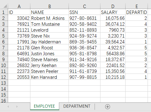
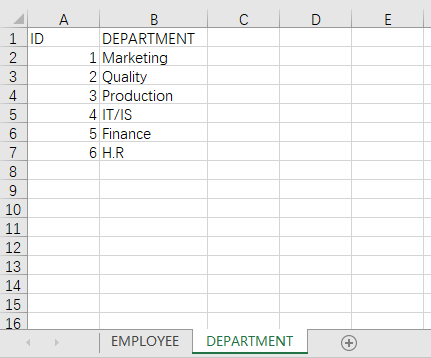
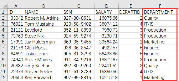
Here is employee salary table on sheet EMPLOYEE. It has only the department IDs in DEPARTID column. This is insufficient for department-related data checking and report building. Fortunately we also have a department information table on sheet DEPARTMENT. Now we want to find the matching ID from the department information table for each DEPARTID in the employee salary table and copy the corresponding department name (which is stored in DEPARTMENT column) to the employee salary table.
Below is salary.xlsx recording employee salaries:
The expected result:
This is the simplest join. VLOOKUP function can implement it well. But there are some points you need to pay more attention. VLOOKUP function needs to know the relative position of the column to be searched and the column to be returned when it performs the lookup. If a column is inserted or deleted between them, the formula should be adjusted. The function also requires that the column to be searched be the first of a table. If the to-be-returned column is before the to-be-searched column, we should first adjust their order.
There are no such problems with SPL because the language accesses columns by names:
A |
B |
|
1 |
=file("salary.xlsx").xlsimport@t() |
/Import the salary table on sheet 1 that has column headers |
2 |
=file("salary.xlsx").xlsimport@t(;"DEPARTMENT") |
/Import the department table on sheet DEPARTMENT |
3 |
=A1.join(DEPARTID,A2:ID,DEPARTMENT) |
/Perform foreign-key-based join on the two table sequences, that is, match salary table’s DEPARTID field to the department table’s ID field and get the corresponding DEPARTMENT field from the latter |
4 |
=file("out.xlsx").xlsexport@t(A3) |
/Export the joining result to another Excel file |
II. multi-column association
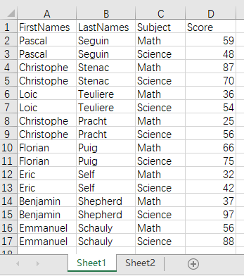
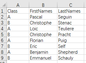
If the source file doesn’t have a primary key like ID, you need multiple columns to do the matching. In the following student score table, the student’s first name and last name are recorded in different columns. To summarize scores by class, we need to find the class each student belongs to according to the first name and last name.
Below is scores.xlsx:
The expected result:
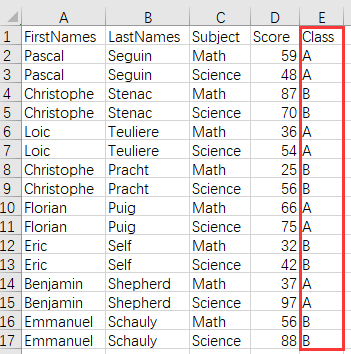
VLOOKUP function performs lookup by searching the first column of a table and one value at a time. The “first” is a must. But searching multiple columns at one time makes VLOOKUP impossible. An alternative is to combine the to-be-searched columns into one auxiliary column using textjoin and perform the lookup by searching the auxiliary column. The target table needs to perform a same join operation too. These preparatory operations make the code even more complicated.
Without the help of an intermediate auxiliary column, SPL can access columns through their names:
A |
B |
|
1 |
=file("scores.xlsx").xlsimport@t() |
/Import the score table on sheet 1 that has column headers |
2 |
=file("scores.xlsx").xlsimport@t(;"Sheet2") |
/Import the class table on sheet 2 |
3 |
=A1.join(FirstNames:LastNames,A2:FirstNames:LastNames,Class) |
/Perform foreign-key-based join on the two table sequences, that is, match score table’s FirstNames field and LastNames field to the corresponding field in class table and get the Class field from the latter |
4 |
=file("out.xlsx").xlsexport@t(A3) |
III. One-to-one association
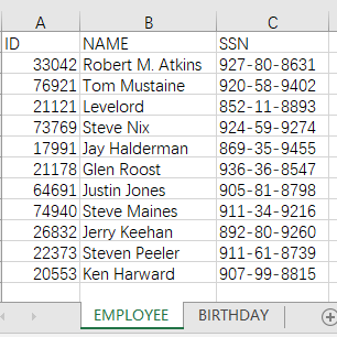
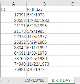
To handle a wide table having a lot of fields, we often need to split the fields to store them in smaller tables having same primary key values. The employee table and birthday table are such small tables. Now we need to associate them through ID field to check the whole employee information.
Below is employee.xlsx:
The expected result:
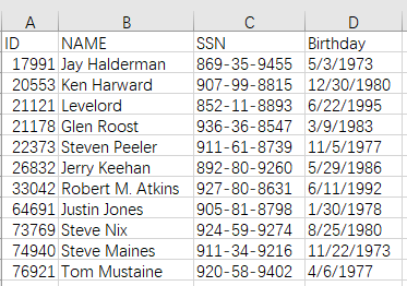
It’s equally complicated to handle a one-to-one association with VLOOKUP because of position problem. Particularly when there are more than two to-be-joined sheets, and VLOOKUP has to implement a join over two tables each time – since it cannot handle a join over more tables at a time, the script will be even more complicated.
SPL can process multiple tables and multiple associated columns at once:But, SPL can handle the association between multiple columns across multiple tables at once:
A |
B |
|
1 |
=file("employee.xlsx").xlsimport@t() |
/Import the employee table on sheet 1 that has column headers |
2 |
=file("employee.xlsx").xlsimport@t(;"BIRTHDAY") |
/Import the birthday table on sheet BIRTHDAY |
3 |
=join(A1:Employee,ID;A2:Birthday,ID).new(Employee.ID,Employee.NAME,Employee.SSN,Birthday.Birthday) |
/Perform foreign-key-based join on the two table sequences, that is, match their ID fields, and generate a new table sequence consisting of the desired fields |
4 |
=file("out.xlsx").xlsexport@t(A3) |
Different from the A.join operation in the previous example, here we use new() function to get the desired fields.
VLOOKUP performs the join based on the table on the left, which is the left join. A left join returns all records from the left table even if there are no matches in the right table and uses empty values to replace missing values. For a one-to-one association, however, we want to have an effect of inner join and full join. An inner join returns only records that have matches and delete those that haven’t. To do this in VOLLOKUP, we need to delete records containing empty values from the joining result. A full join returns all matching records from both tables whether the other table matches or not. VLOOKUP cannot implement a full join directly. It has to do the join one by one, concatenate the result sets and then delete the duplicate records. That is very complicated.
Below is employees.xlsx:
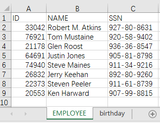
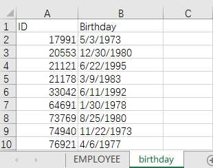
An examine shows that the employee table doesn’t have IDs 21121,73769 and 17991 and that the birthday table doesn’t include IDs 22373 and 26832.
1. Left join
To do a left join is to return all records in the employee table, even the corresponding record in the birthday table have empty values under Birthday column. The target result is as follows:
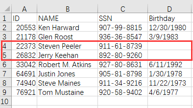
To do the left join in SPL, you just need to use @1 option with the join() function. Then A3’s code in the previous script should be changed to the following:
=join@1(A1:Employee,ID;A2:Birthday,ID).new(Employee.ID,Employee.NAME,Employee.SSN,Birthday.Birthday)
2. Inner join
The join() function works alone to perform an inner join. An inner join returns records that have matches in both tables.
The target result:
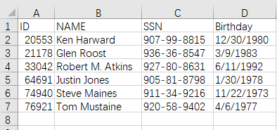
To do an inner join, A3’s code in the SPL script will be:
=join(A1:Employee,ID;A2:Birthday,ID).new(Employee.ID,Employee.NAME,Employee.SSN,Birthday.Birthday)
3. Right join
To do a right join is to return all records in the birthday table even there are empty values in the other table. Below is the target result:
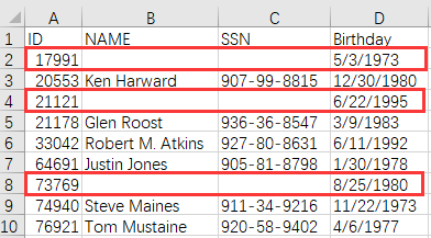
A right join is the left join of two tables in reversed order. An ID should be retrieved based on the right table Birthday; otherwise the value will be empty. In this case, the SPL code in A3 will be as follows:
=join@1(A2:Birthday,ID;A1:Employee,ID).new(Birthday.ID,Employee.NAME,Employee.SSN,Birthday.Birthday)
4. Full join
A full join is equivalent to the union of the result set of the left join and that of the right join. Below is the target result:
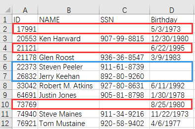
@f option is used with the join() function to perform a full join. The ID will be retrieved from the table where a match can be found. So the SPL code in A3 should be:
=join@f(A2:Birthday,ID;A1:Employee,ID).new(if(Birthday==null,Employee.ID,Birthday.ID):ID,Employee.NAME,Employee.SSN,Birthday.Birthday)
IV. One-to-many association
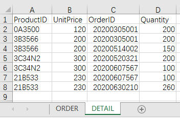
In real-world businesses, an order table often has several detailed data sub tables. In such cases, one order record corresponds to multiple detailed data records, as shown by the ORDER table and DETAIL table. That is the one-to-many association. Now we need to relate each order to its detailed data through OrderID for the convenience of summing the order amounts by dates.
Below is orders.xlsx:
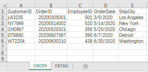
The target result:
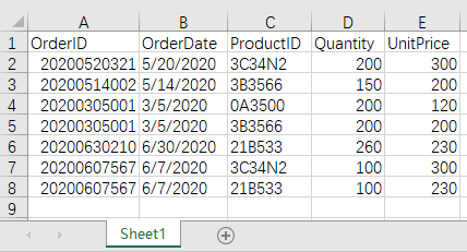
The one-to-many association involves adding records to the left table after matches are found in the right table. You cannot achieve this using the left join. So you can’t use VLOOKUP that performs the lookup based on the left table to do this. As a left join can’t be used, a full join is also impossible. An inner join is feasible if we make the DETAIL table the source table to find the matches and then remove records where the orderIDs are empty.
SPL makes it simple by specifying the joining fields without considering the association relationship:
A |
B |
|
1 |
=file("orders.xlsx").xlsimport@t() |
/Import the ORDER table on sheet 1 that has column headers |
2 |
=file("orders.xlsx").xlsimport@t(;"DETAIL") |
/Import the detailed data on sheet DETAIL |
3 |
=join(A1,OrderID;A2,OrderID).new(_1.OrderID,_1.OrderDate,_2.ProductID,_2.Quantity,_2.UnitPrice) |
/Join tables by the specified fields and get desired field to generate a new table sequence |
4 |
=file("out.xlsx").xlsexport@t(A3) |
SPL uses join() function to implement a join of one-to-many association or one-to-one association by specifying the joining fields. It uses the same method to perform different types of joins.
V. Non-equi-association
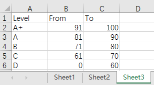
In the previous examples, we perform different types of joins according to whether the joining field values match. There is another type of comparison to see whether records in two tables match. Take the score table in the above as an example. Now we need to rate scores according to the specified ranges instead of checking whether the score in the right table is equal.
Below is the score level table:
The target result:
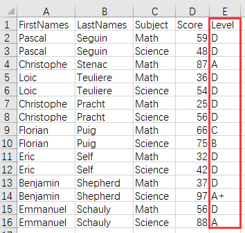
It’s similar to the many-to-one association though the type of joining condition is different. VLOOKUP function will sort the conditional ranges in ascending order and then employ fuzzy matching technique to compare records in the two tables.
SPL offers methods to perform the non-equi-association, too:
A |
B |
|
1 |
=file("scores.xlsx").xlsimport@t() |
/Import the ORDER table on sheet 1 that has column headers |
2 |
=file("scores.xlsx").xlsimport@t(;"Sheet3") |
/Import the level table on sheet 3 |
3 |
=xjoin(A1:Score;A2:Level,A2.From<Score.Score && Score.Score<A2.To) |
/Perform cross product using xjoin and get eligible records by the filtering conditions |
4 |
=A3.new(Score.FirstNames,Score.LastNames,Score.Subject,Score.Score,Level.Level) |
/Return a new table sequence made up of desired fields after matching |
5 |
=file("out.xlsx").xlsexport@t(A4) |
The script performs a full cross product using xjoin and then deletes the ineligible records according to the filtering conditions.
Find more examples in SPL Cookbook.
SPL Official Website 👉 https://www.scudata.com
SPL Feedback and Help 👉 https://www.reddit.com/r/esProcSPL
SPL Learning Material 👉 https://c.scudata.com
SPL Source Code and Package 👉 https://github.com/SPLWare/esProc
Discord 👉 https://discord.gg/2bkGwqTj
Youtube 👉 https://www.youtube.com/@esProc_SPL


