Multidimensional Analysis Backend Practice 7: Boolean Dimension and Binary Dimension
Abstract
This series of articles explain how to perform multidimensional analysis (OLAP) in steps with detailed samples. Click to learn more in Multidimensional Analysis Backend Practice 7: Boolean Dimension and Binary Dimension. Multidimensional Analysis Backend Practice 7: Boolean Dimension and Binary Dimension
Aim of practice
This issue aims to achieve boolean dimension and binary dimension on the basis of the optimization in previous issues (especially the sequence numberization of branch department dimension in the last issue), thus further improving the calculation speed.
The steps of practice are:
1. Prepare the customer table: modify the code in previous issues to convert the branch department and job of the customer table to boolean dimensions and the eight flag bits to binary dimensions.
2. Access the customer table: modify the query code to improve the computation speed.
To realize the multidimensional analysis calculation requirements of verifying boolean dimensions, we will use the customer data stored in customerEnum.ctx as shown in the following picture:

The city field stores the cities where the customers live, and its value range is from 1 to 660.
The calculation requirements can be described in the following SQL1 of Oracle:
select department_id,job_id,to_char(begin_date,'yyyymm') begin_month ,sum(balance) sum,count(customer_id) count
from customer
where city in (36,37,38,39,40,60,61,62,63,64,65,66,67,68,69,640,641,642,643,644,645,646,647,648,649,650,651,652,653,654,655,656,657,658,659,660)
group by department_id,job_id,to_char(begin_date,'yyyymm') begin_month
The multidimensional analysis calculation requirements of verifying binary dimensions can be described in SQL2:
select department_id,job_id,to_char(begin_date,'yyyymm') begin_month ,sum(balance) sum,count(customer_id) count
from customer
where flag1=1 and flag2=1 and flag3=1 and flag5=1 and flag6=1 and flag8=1
group by department_id,job_id,to_char(begin_date,'yyyymm') begin_month
Prepare data
Boolean dimensions can directly adopt to the storage scheme of customerEnum.ctx.
Binary dimensions are represented by converting the eight flag bits, form flag1 to flag8, to the 8 bits of an integer. Continue to write etl.dfx to generate composite table file customerFlag.ctx after converting customerDept.ctx of the last issue. The code sample is:
|
A |
1 |
=file("data/customerDept.ctx").open().cursor() |
2 |
=A1.new(department_id,job_num,employee_id,begin_date,customer_id,first_name,last_name,phone_number,job_title,balance,department_name,vip_id,credit_grade,bits(flag8,flag7,flag6,flag5,flag4,flag3,flag2,flag1):flag) |
3 |
=file("data/customerFlag.ctx").create@y(#department_id,#job_num,#employee_id,#begin_date,#customer_id,first_name,last_name,phone_number,job_title,balance,department_name,vip_id,credit_grade,flag) |
4 |
=A3.append(A2) |
A1: open the composite table file customerDept.ctx, and created a cursor based on it.
A2: generate a new cursor, and use the bits function to represent the original 8 fields as the 8 bits of an integer. For example, flag1 to flag8 are 1, 0, 1, 1, 0, 1, 1, 1, which is 237 as decimal integer and 1110 1101 in binary, the 8 bits corresponding to flag1 to flag8 from right to left respectively.
When the data volume is 100 million, compare the exported composite table file with the composite table file in last issue as follows:
Number of issue |
Size of file |
Description |
Note |
Six |
2.6GB |
Without binary dimension optimization |
|
Seven |
2.4GB |
Binary dimension optimization done |
As seen in the above table, the file size decreases by 0.2GB after optimizing the data type. The more the number of binary dimensions, the more significantly the optimized file becomes smaller. Smaller files will reduce the amount of data read from the disk, thus improving the performance to some extent. When calculating files in columnar storage, the number of fields to be read will decrease, which is more helpful to the performance improvement.
Multidimensional analysis calculation
1. Boolean dimensions
The SPL code consists of olap.dfx and customerEnum.dfx, the former is the entry of calling and the given parameters are arg_table and arg_json, the latter is used to parse arg_json.
The value of arg_table is customerEnum.
The value of arg_json is:
{
       aggregate:
              [
                     {func:"sum",field:"balance",alias:"sum"},
                 {func:"count",field:"customer_id",alias:"count"}
              ],
       group:
              ["department_id","job_id","begin_yearmonth"],
       slice:
              [
                     {dim:"city",
                     value:[36,37,38,39,40,60,61,62,63,64,65,66,67,68,69,640,641,642,
                      643,644,645,646,647,648,649,650,651,652,653,654,655,656,
                            657,658,659,660]
                     }
               ]
}
The code of customerEnum.dfx is:
A |
B |
C |
|
1 |
Func |
||
2 |
if A1.bool!=null |
return string(A1.bool)/"("/A1.dim/")" |
|
3 |
else if A1.value==null |
return "between("/A1.dim/","/A1.interval(1)/":"/A1.interval(2)/")" |
|
4 |
else if ifa(A1.value) |
return string(A1.value)/".contain("/A1.dim/")" |
|
5 |
else if ifstring(A1.value) |
return A1.dim/"==\""/A1.value/"\"" |
|
6 |
else |
return A1.dim/"=="/A1.value |
|
7 |
=json(arg_json) |
=date("2000-01-01") |
|
8 |
=A7.aggregate.(~.func/"("/~.field/"):"/~.alias).concat@c() |
||
9 |
=A7.group.(if(~=="job_id","job_num",~)) |
||
10 |
=A9.(if(~=="begin_yearmonth","begin_date\\100:begin_yearmonth",~)).concat@c() |
||
11 |
=A7.aggregate.(field) |
=A9.(if(~=="begin_yearmonth","begin_date",~)) |
|
12 |
=(A11|C11).id().concat@c() |
||
13 |
=[] |
||
14 |
for A7.slice.derive(null:bool) |
if A14.dim=="begin_date" && A14.value!=null |
>A14.value=int(interval@m(C7,eval(A14.value))*100+day(eval(A14.value))) |
15 |
else if A14.dim=="begin_date" && A14.value==null |
=A14.interval.(~=int(interval@m(C7,eval(~))*100+day(eval(~)))) |
|
16 |
else if A14.dim=="job_id" |
>A14.dim="job_num" |
|
17 |
>A14.value=A14.value.(job.pos@b(~)) |
||
18 |
else if A14.dim=="city" |
=to(660) |
|
19 |
=C18.(A14.value.contain(#)) |
||
20 |
=A14.bool=C19 |
||
21 |
else if like(A14.dim, "flag?") |
>A14.value=int(A14.value) |
|
22 |
=[func(A1,A14)] |
>A13|=B22 |
|
23 |
=A7.group|A7.aggregate.(alias) |
=A23(A23.pos("job_id"))="job(job_num):job_id" |
|
24 |
=A23(A23.pos("begin_yearmonth"))="month@y(elapse@m(date(\""/C7/"\"),begin_yearmonth)):begin_yearmonth" |
||
25 |
=A23(A23.pos("begin_date"))="elapse@m(B4,begin_date\\100)+(begin_date%100-1):begin_date" |
||
26 |
return A12,A8,A10,A13.concat("&&"),A23.concat@c() |
||
Area from A1 to C6 is subprogram which only executes when being called. We will explain them in the order of execution for the sake of better illustration.
A7: parse arg_json to a table sequence and the return result is a nested multi-layer table sequence as follows:

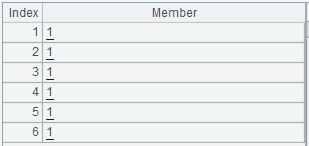
The “aggregate” in it is:

The “group” is:

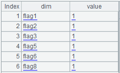
The “slice” is:

C7: define the beginning date as 2000-01-01 for the conversion of date values in parameters and results.
A8: first calculate “aggregate” to colon-concatenated string sequences and then concatenate the sequences to a string with a comma: sum(balance):sum,count(customer_id):count, i.e., the aggregate expression.
A9: replace the job_id in “group” with job_num.
A10: replace the begin_yearmonth in A8 with expression begin_date\100:begin_yearmonth. Then concatenate the members in A8 to a string with commas: department_id,job_num,begin_date\100:begin_yearmonth, i.e., the grouping expression.
A11: get the “field” in “aggregate”, that is, all the field names used in the aggregate expression.
C11: replace the begin_yearmonth in “group” with begin_date, and the results are all the field names used in the grouping expression.
A12: union A10 and C10 and then concatenate them as a string to get all the required field names for this calculation: balance, begin_date, customer_id, department_id, and job_num.
A13: define an empty sequence which prepares to store the slice (filtering conditions) expression sequence.
A14: loop through A7.slice with an added “bool” field and the loop body is B14 to C22 in which from B14 to C21 is the optimization conversion to the “value” or “interval” of “slice”.
B14: if the “dim” of A14 (the current slice) is begin_date and the “value” is not null, that is, the begin_date equals to the specified date. For example, begin_date==date("2010-11-01"). In this case, C14 calculates the converted integer value of date("2010-11-01") and assigns it to the “value” of A14.
B15: if the “dim” of A14 is begin_date and the “value” is null, that is, the begin_date is between two dates. For example: begin_date is between date("2002-01-01") and date("2020-12-31"). In this case, C15 calculates the converted integer values of those two dates and assigns them to two members of “interval” in A13.
B16: if the “dim” of A14 is job_id, that is, job_id is an enumeration value, for example, ["AD_VP","FI_MGR","AC_MGR","SA_MAN","SA_REP"].contain(job_id). In this case, C16 converts the “dim” of A14 to job_num and C17 converts the enumeration value “value” of A14 to the position in the sequence of global variable “job”, i.e., job_num integer sequence. For example: [5,7,2,15,16].
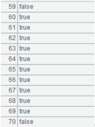
B18: if the “dim” of A14 is city, C18 generates a sequence with the number of city dimension as its length, and C19 uses the “value” (“city” enumeration value) of A14 to assign the corresponding members of C19 as true and others as false. C19 is the boolean dimension sequence, and the results are as follows:

C20: assign C19 to the “bool” field of A14.
B21: if the “dim” of A14 is flag1, flag2, ..., flag8, that is, the flag bit equals to “1” or “0”. In this case, C21 converts the “value” of A14 from strings to integers.
B22: take the result of B14 to C21, which converts the “bool”, “value” or “interval” of “slice” for performance optimization, as parameter to call subprogram A1.
The subprogram A1 (from B2 to B6) is basically identical to the func code in the second article with only B2 and C2 added. B2 verifies if the “bool” filed is null, if not, then C2 will generate and return the boolean dimension expression. For example: [false,true,false…](city), which is used to take the values of “city” field as sequence numbers to find the members at the corresponding positions in the boolean dimension sequence. If the result is true, then it is a record that meets the enumeration condition, otherwise it is a record that does not meet the condition.
C22: append the return result of func A1 to A13. Continue the loop in A14 until it is over. And the sequence of slice expressions is well prepared.
A23: prepare the conversion expression of result set display value from here. Concatenate A6.group with A6.aggregate.alias sequence as follows:

C23: replace the job_id in A23 with conversion statement which is used to convert the job_num in result set to job_id.
A24: replace the begin_yearmonth in A23 with conversion statement which is used to convert the begin_yearmonth in grouping fields from integers to yyyymm.
A25: replace the begin_date in A23 with conversion statement which is used to convert the integer date values in grouping fields to date type. At this point A23 is the prepared result set display value conversion expression:

A26: return A12, A8, A10, A13.concat("&&"), and A23.concat@c() respectively as:
The field names used in the calculation: balance, begin_date, customer_id, department_id, job_num
The aggregate expression: sum(balance):sum,count(customer_id):count
The grouping expression: department_id,job_num,begin_date\100:begin_yearmonth
The slice expression:
[false,false,false,false,false,false,false,false,false,false,… false,false,true,true,true,true,
true,true,true,true,true,true,true,true,true,true,true,true,true,true,true,true,true](city)
The result set display value conversion expression:
department_id,job(job_num):job_id,month@y(elapse@m(date("2000-01-01"),begin_yearmonth)):begin_yearmonth,sum,count
Boolean dimension optimization has no special requirement for olap.dfx, and the code is:
A |
|
1 |
=call(arg_table/".dfx",arg_json) |
2 |
=file("data/"/arg_table/".ctx").open() |
3 |
=A2.cursor@m(${A1(1)};${A1(4)};2) |
4 |
=A3.groups(${A1(3)};${A1(2)}) |
5 |
=A4.new(${A1(5)}) |
6 |
return A5 |
A3: what actually executes is the code after boolean dimension optimization:
=A2.cursor@m(balance,begin_date,customer_id,department_id,job_num; [false,false,false,false,false,false,false,false,false,false,… false,false,true,true,true,true,true,true,true,true,true,true,true,true,true,true,true,true,true,true,true,true,true](city);2), which is used to take the values of “city” fields as sequence numbers to find the members at the corresponding positions in the boolean dimension sequence. If the result is true, then it is a record that meets the enumeration condition, otherwise it is a record that does not meet the condition.
The Java code used to call the SPL code remains unchanged compared to last issue as long as the calling parameters are adjusted.
The total execution time of Java code plus the backend calculation of return results is as follows:
Calculation method |
Single-thread |
Two-thread |
Note |
Without boolean dimension optimization |
11 seconds |
6 seconds |
|
Boolean dimension optimization |
6 seconds |
4 seconds |
It can be seen from the above table that boolean dimension optimization can improve the calculation performance.
2. Binary dimension
The SPL code consists of olap.dfx and customerFlag.dfx, the former is the entry of calling and the given parameters are arg_table and arg_json, the latter is used to parse arg_json.
The value of arg_table is customerFlag.
The value of arg_json is:
{
       aggregate:
              [
                     {func:"sum",field:"balance",alias:"sum"},
                 {func:"count",field:"customer_id",alias:"count"}
              ],
       group:
              ["department_id","job_id","begin_yearmonth"],
       slice:
              [
                     {dim:"flag1",value:"1"},
                     {dim:"flag2",value:"1"},
                     {dim:"flag3",value:"1"},
                     {dim:"flag5",value:"1"},
                     {dim:"flag6",value:"1"},
                     {dim:"flag8",value:"1"}
               ]
}
The code of customerFlag.dfx is as follows:
A |
B |
C |
|
1 |
func |
||
2 |
if A1.bool!=null |
return string(A1.bool)/"("/A1.dim/")" |
|
3 |
else if A1.value==null |
return "between("/A1.dim/","/A1.interval(1)/":"/A1.interval(2)/")" |
|
4 |
else if ifa(A1.value) |
return string(A1.value)/".contain("/A1.dim/")" |
|
5 |
else if ifstring(A1.value) |
return A1.dim/"==\""/A1.value/"\"" |
|
6 |
else |
return A1.dim/"=="/A1.value |
|
7 |
=json(arg_json) |
=date("2000-01-01") |
|
8 |
=A7.aggregate.(~.func/"("/~.field/"):"/~.alias).concat@c() |
||
9 |
=A7.group.(if(~=="job_id","job_num",~)) |
||
10 |
=A9.(if(~=="begin_yearmonth","begin_date\\100:begin_yearmonth",~)).concat@c() |
||
11 |
=A7.aggregate.(field) |
=A9.(if(~=="begin_yearmonth","begin_date",~)) |
|
12 |
=(A11|C11).id().concat@c() |
||
13 |
=A7.slice.select(like(dim,"flag?")) |
=A13.derive(int(right(dim,1)):num) |
=to(8).("0") |
14 |
=B13.(C13(num)=value) |
=bits(C13.rvs()) |
="and(flag,"/B14/")=="/B14 |
15 |
=[] |
=A7.slice\A13 |
|
16 |
for B15 |
if A16.dim=="begin_date" && A16.value!=null |
>A16.value=int(interval@m(C7,eval(A16.value))*100+day(eval(A16.value))) |
17 |
else if A16.dim=="begin_date" && A16.value==null |
=A16.interval.(~=int(interval@m(C7,eval(~))*100+day(eval(~)))) |
|
18 |
else if A16.dim=="job_id" |
>A16.dim="job_num" |
|
19 |
=A16.value.(job.pos@b(~)) |
||
20 |
=[func(A1,A16)] |
>A15|=B20 |
|
21 |
=A7.group|A7.aggregate.(alias) |
=A21(A21.pos("job_id"))="job(job_num):job_id" |
|
22 |
=A21(A21.pos("begin_yearmonth"))="month@y(elapse@m(date(\""/C7/"\"),begin_yearmonth)):begin_yearmonth" |
||
23 |
=A21(A21.pos("begin_date"))="elapse@m(B4,begin_date\\100)+(begin_date%100-1):begin_date" |
||
24 |
return A12,A8,A10,(A15|C14).concat("&&"),A21.concat@c() |
||
Area from A1 to A12 is not changed compared to customerEnum.dfx.
A13: filter out the “dim” starting with “flag” in the slice filtering condition A7.slice as follows:

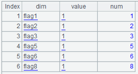
B13: add one “num” column in A13, take the last number of “dim” and convert it to integer:

C13: create a sequence whose length is 8, each member of which is the string “0”.
A14: loop through B13, and set the corresponding positions of C13 as value “1”.

B14: invert the order of members in C13 and use the bits function to calculate the corresponding integer value: 237, i.e., 1011 0111 in binary, which corresponds to the values of original flag1 to flag8 from right to left, respectively.
C14: use B14 to concatenate strings and generate the bitwise AND expression: and(flag,237)==237, which will be part of the filtering expression later.
A15: define an empty sequence which prepares to store slice (filtering condition) expression sequence.
B15: remove A13 from A7.slice to get the slice conditions other than flag1 to flag8.
A16: start looping though B15 and process the slice conditions other than flag1 to flag8 during the loop.
A16-A23: the code is exactly the same as that of customerEnum.dfx.
A24: return A12, A8, A10, A13.concat("&&"), and A23.concat@c() respectively as:
The fields used in the calculation: balance, begin_date, customer_id, department_id, and job_num
The aggregate expression: sum(balance):sum,count(customer_id):count
The grouping expression: department_id,job_num,begin_date\100:begin_yearmonth
The slice expression: and(flag,237)==237
The result set display value conversion expression:
department_id,job(job_num):job_id,month@y(elapse@m(date("2000-01-01"),begin_yearmonth)):begin_yearmonth,sum,count
Binary dimension optimization also has no special requirement for olap.dfx, and the code is:
A |
|
1 |
=call(arg_table/".dfx",arg_json) |
2 |
=file("data/"/arg_table/".ctx").open() |
3 |
=A2.cursor@m(${A1(1)};${A1(4)};2) |
4 |
=A3.groups(${A1(3)};${A1(2)}) |
5 |
=A4.new(${A1(5)}) |
6 |
return A5 |
A3: what actually executes is the code after binary dimension optimization:
=A2.cursor@m(balance,begin_date,customer_id,department_id,job_num;and(flag,237)==237;2), which is used to perform bitwise AND between the value of “flag” field and 237. And if the result is 237, it is a record that meets the enumeration condition, otherwise, it is a record that does not meet the condition.
The Java code used to call the SPL code remains unchanged compared to last issue as long as the calling parameters are adjusted.
The total execution time of Java code plus the backend calculation of return results is as follows:
Calculation method |
Single-thread |
Two-thread |
Note |
Without binary dimension optimization |
16 seconds |
9 seconds |
|
Binary dimension optimization |
7 seconds |
4 seconds |
It can be seen from the above table that binary dimension optimization can also improve the calculation performance.
SPL Official Website 👉 https://www.scudata.com
SPL Feedback and Help 👉 https://www.reddit.com/r/esProc_SPL
SPL Learning Material 👉 https://c.scudata.com
SPL Source Code and Package 👉 https://github.com/SPLWare/esProc
Discord 👉 https://discord.gg/cFTcUNs7
Youtube 👉 https://www.youtube.com/@esProc_SPL


Chinese version