SPL provides programmers with powerful index mechanisms and various query functions for objects in different scenarios, which can significantly improve the query performance if used well.

 

1. Key value search

1.1 Table sequence

We first generate a piece of simulation data of “call records” to compare the impacts of different query functions on the query performance of table sequence. The code for creating the simulation data is as follows:

	A
1	=5000000.new(13800000000+~:Subscriber,datetime(1547123785410+rand(864000000)):Time,rand(3600)+1:Length,rands("TF",1):isLocal)
2	=file("btx/voiceBill.btx").export@b(A1)

[Code 1.1.1]

 

Some of the data are:

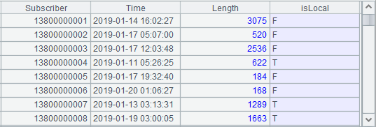
[Figure 1.1.1]

 

To query the table sequence, we usually think of the A.select() function whose effects are shown in the following code:

	A	B
1	=file("btx/voiceBill.btx").import@b()	/load the data of the file to generate a table sequence
2	=now()	/the current time
3	=A1.select(Subscriber==13800263524)	/use A.select() function to query
4	=interval@ms(A2,now())	/the time spent in the query

[Code 1.1.2]

 

The query time is 80 milliseconds.

 

We can use the A.find() function to query the key values of the table sequence. And the code sample is:

	A	B
1	=file("btx/voiceBill.btx").import@b()	/load the data of the file to generate a table sequence
2	>A1.keys(Subscriber)	/set Subscriber as the primary key
3	>A1.index()	/create index
4	=now()	/the current time
5	=A1.find(13800263524)	/use the A.find() function to search
6	=interval@ms(A4,now())	/the time spent in the query

[Code 1.1.3]

 

The time used is 1 millisecond.

 

This is because we can specify a certain field or some fields as the primary key in the table sequence of esProc and the particular function can be used to perform the search based on the primary key. For example, the find function in A5 of Code 1.1.3 not only simplifies the syntax but also boosts the calculation efficiency greatly.

 

We can also use the A.find@k() function to perform batch key value search when there are many key values. And the code sample is:

	A	B
1	=file("btx/voiceBill.btx").import@b()	/load the data of the file to generate a table sequence
2	>A1.keys(Subscriber)	/set Subscriber as the primary key
3	>A1.index()	/create index
4	=A1(50.(rand(A1.len())+1)).(Subscriber)	/retrieve 50 values from Subscriber randomly
5	=now()	/the current time
6	=A1.find@k(A4)	/use A.find@k() function to perform batch key value search
7	=interval@ms(A5,now())	/the time spent in searching

[Code 1.1.4]

 

It is worth noting that we should create the primary key in advance when using the A.find() function, otherwise it will report an error of “missing primary key”.

 

The reason why the function of primary key value search can efficiently improve the calculation is because it creates index on the primary key of the table sequence. In Code 1.1.4, the average query time is 1,400 milliseconds without index; while the query time is less than 1 millisecond with index created.

 

The larger the data in the table sequence, the more searching operations are required, and the more significant the improvement in efficiency.

 

When the query condition corresponds to several keys, the code sample is:

	A	B
1	=file("btx/voiceBill.btx").import@b()	/load the data of the file to generate a table sequence
2	>A1.keys(Subscriber,isLocal)	/set Subscriber and isLocal as the primary keys
3	>A1.index()	/create index
4	=[[13800000002,"F"],[13802568478,"F"]]	/concatenate multiple keys to a sequence
5	=now()	/the current time
6	=A1.find@k(A4)	/use the A.find@k() function to perform batch key value search on A4
7	=interval@ms(A5,now())	/the time spent in the query

[Code 1.1.5]

 

The switch/join function also needs to find records in the table sequence based on the primary key value, which will automatically create index on the dimension table. The multi-thread fork function will automatically create an index on the corresponding dimension table in each thread if the index has not been created beforehand, but this processing will definitely consume more memory at runtime, resulting in memory overflow like in Figure 1.1.2. To avoid this situation, a better method is shown in Figure 1.1.3.

[Figure 1.1.2] Every thread in the fork function creates index on its own automatically, which leads to memory overflow.

 

[Figure 1.1.3] It creates index on the dimension table before the fork function executes.

 

1.2 Bin file

 

To search an ordered bin file, we can use the f.select() function to perform the binary search. This function also supports the batch search, and the following example is using the f.select() function to perform the batch search based on bin file:

	A
1	=5000000.new(13800000000+~:Subscriber,datetime(1547123785410+rand(864000000)):Time,rand(3600)+1:Length,rands("TF",1):isLocal)
2	=file("btx/voiceBill@z.btx").export@z(A1)

[Code 1.2.1]

 

Code 1.2.1 is to create the bin file voiceBill@z.btx. And Subscriber is ordered obviously.

 

	A	B
1	=file("btx/voiceBill@z.btx")
2	=50.(13800000000+rand(5000000)+1).id()	/retrieve 50 Subscriber out of 5 million randomly, de-duplicate and sort them
3	=now()	/the current time
4	=A1.iselect@b(A2,Subscriber)	/use the binary search function, f.iselect(), to batch search the bin file
5	=A4.fetch()
6	=interval@ms(A3,now())	/the time spent in the query

[Code 1.2.2]

 

In Code 1.2.2, since f.iselect()is a binary search function, we should note that A2, as the search sequence, should be ordered just as the id number of the bin file. Also, here @b option does not mean the binary search but to load the bin file exported by the f.export function. And @z option is used to export the bin file, otherwise the f.iselect() function will report an error when querying the bin file.

 

Suppose the total amount of data is N, then the time complexity of binary search is logN (2 as the base), and the performance improvement becomes more significant as the data amount gets larger.

 

1.3 Composite table

 

There are T.find()and T.find@k() functions in composite table. They are similar to those in table sequence and can achieve key value search in an efficient way, quite suitable for the scenarios of searching a small number of records in a big dimension table. For example:

	A	B
1	=file("ctx/voiceBill.ctx").create(#Subscriber,Time,Length,isLocal)
2	for 5000	=to((A2-1)*10000+1,A2*10000).new(13800000000+~:Subscriber,datetime(1547123785410+rand(864000000)):Time,rand(3600)+1:Length,rands("TF",1):isLocal)
3		=A1.append(B2.cursor())

[Code 1.3.1]

 

Code 1.3.1 is to create the composite table file voiceBill.ctx, in which Subscriber is the dimension of the composite table.

 

	A	B
1	=file("ctx/voiceBill.ctx").open()	/open the composite table
2	=13801701672	/one Subscriber value of the composite table data
3	=now()	/the current time
4	=A1.cursor().select(Subscriber==A2).fetch()	/use cs.select() function to query the composite table
5	=interval@ms(A3,now())	/the time spent in the query

[Code 1.3.2]

 

Code 1.3.2 is to query the composite table using the cs.select() function, and the time is 13,855 milliseconds.

 

	A	B
1	=file("ctx/voiceBill.ctx").open()	/open the composite table
2	=13801701672	/one Subscriber value of the composite table data
3	=now()	/the current time
4	=A1.find(A2)	/use T.find() function to query the composite table
5	=interval@ms(A3,now())	/the time spent in the query

[Code 1.3.3]

 

Code 1.3.3 is to query the composite table using the T.find() function, and the time is 77 milliseconds.

 

According to the comparison, for the composite table with dimensions, we can use the T.find() function similar to table sequence to perform single or batch key value search, which is much more efficient than fetching data from the filtered cursor.

 

2. Index search

 

We can create three kinds of index on the composite table, which is applicable to different situations respectively:

1. hash index is suitable for single value search such as the enumeration type;

2. Sorted index is suitable for interval search such as number, date and time types;

3. Full-text index is suitable for fuzzy search such as string type.

 

In the following, we’ll create the composite table whose data type includes all the three index mentioned above:

	A	B
1	=file("ctx/voiceBillDetail.ctx").create(#Subscriber,Time,Length,isLocal,City,Company)
2	=file("info/city_en.txt").import@i()	=A2.len()
3	for 5000	=to((A3-1)*10000+1,A3*10000).new(13800000000+~:Subscriber,datetime(1547123785410+rand(864000000)):Time,rand(3600)+1:Length,rands("TF",1):isLocal,A2(rand(B2)+1):City,rands("ABCDEFGHIJKLMNOPQRSTUVWXYZ",14)+"  Co. Ltd":Company)
4		=A1.append(B3.cursor())

[Code 2.1]

 

The first ten records of the composite table created in Code 2.1 are as follows:

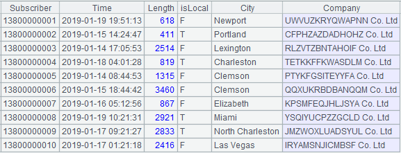
[Figure 2.1]

 

 

	A	B
1	=file("ctx/voiceBillDetail.ctx").open()	/open the composite table
2	=A1.index(subscriber_idx;Subscriber)	/phone number of the subscriber, sorted index on numbers
3	=A1.index(time_idx;Time)	/starting point of the call, sorted index on numbers
4	=A1.index(length_idx;Length)	/call duration, sorted index on numbers
5	=A1.index(city_idx:1;City)	/city, hash index on enumeration
6	=A1.index@w(company_idx;Company)	/company, full-text index on strings

[Code 2.2]

 

Different types of index are created in Code 2.2 according to the characteristics of data in each column. The index and composite table file are shown in Figure 2.2:

[Figure 2.2]

 

esProc can automatically identify conditions to create an appropriate index, including equivalence, interval, and like(“A*”)-type. In the next section, let’s take a look at the effects:

 

Equivalence search

 

	A	B
1	=file("ctx/voiceBillDetail.ctx").open()	/open the composite table
2	=now()	/the current time
3	=A1.icursor(;Subscriber==13834750766,subscriber_idx).fetch()	/query with icursor
4	=interval@ms(A2,now())	/the time spent in the query

[Code 2.3]

 

	A	B
1	=file("ctx/voiceBillDetail.ctx").open()	/open the composite table
2	=now()	/the current time
3	=A1.icursor(;Subscriber==13834750766).fetch()	/query with icursor
4	=interval@ms(A2,now())	/the time spent in the query

[Code 2.4]

 

Code 2.3 is written with the index name, while Code 2.4 is written without the index name. And the time consumption of both is basically the same, around 100 milliseconds.

 

	A	B
1	=file("ctx/voiceBillDetail.ctx").open()	/open the composite table
2	=now()	/the current time
3	=A1.cursor().select(Subscriber==13834750766).fetch()	/query with the ordinary cursor
4	=interval@ms(A2,now())	/the time spent in the query

[Code 2.5]

 

Code 2.5 is to query the same records with the ordinary cursor, which takes about 40 seconds.

 

Interval search

 

	A	B
1	=file("ctx/voiceBillDetail.ctx").open()	/open the composite table
2	=now()	/the current time
3	=A1.icursor(;Subscriber>=13834750766 && Subscriber<=13834750780).fetch()	/query with icursor
4	=interval@ms(A2,now())	/the time spent in the query

[Code 2.6]

 

Code 2.6 is to create sorted index on Subscriber to perform interval search, which takes about 70 milliseconds.

 

	A	B
1	=file("ctx/voiceBillDetail.ctx").open()	/open the composite table
2	=now()	/the current time
3	=A1.cursor().select(Subscriber>=13834750766 && Subscriber<=13834750780).fetch()	/query with the ordinary cursor
4	=interval@ms(A2,now())	/the time spent in the query

[Code 2.7]

 

Code 2.7 is to query the same records with an ordinary cursor, costing around 40 seconds.

 

Fuzzy search

 

	A	B
1	=file("ctx/voiceBillDetail.ctx").open()	/open the composite table
2	=now()	/the current time
3	=A1.icursor(like(Company,"*ABCDE*")).fetch()	/query with icursor
4	=interval@ms(A2,now())	/the time spent in the query

[Code 2.8]

 

Code 2.8 is to create full-text index on Company in order to perform fuzzy search, which costs 1,500 milliseconds approximately.

 

	A	B
1	=file("ctx/voiceBillDetail.ctx").open()	/open the composite table
2	=now()	/the current time
3	=A1.cursor().select(like(Company,"*ABCDE*")).fetch()	/query with the ordinary cursor
4	=interval@ms(A2,now())	/the time spent in the query

[Code 2.9]

 

Code 2.9 is to query the same records with an ordinary cursor, taking around 40 seconds.

 

When the data volume is even larger, for example:

	A	B
1	=file("ctx/employee.ctx")
2	=A1.create(#id,name,sex,city,birthday,salary,level,height,weight,company)
3	=file("info/ming_en_female.txt").import@i()	=A3.len()
4	=file("info/ming_en_male.txt").import@i()	=A4.len()
5	=file("info/xing_en.txt").import@i()	=A5.len()
6	=city=file("info/city_en.txt").import@i()	=A6.len()
7	=salary=20000	/10000~30000
8	=["one","two","three","four","five","six","seven","eight","nine","ten"]	=A8.len()
9	=height=50	/160~210cm
10	=weight=50	/50~100kg
11	=birthtime=946656	/1970~2000
12	for 10000	=to((A12-1)*100000+1,A12*100000).new(~:id,if(rand(2)==0,A3(rand(B3)+1),A4(rand(B4)+1))+" "+A5(rand(B5)+1):name,if(A3.pos(name.array("")(1)),"Female","Male"):sex,A6(rand(B6-1)+1):city,date(rand(birthtime)*long(1000000)):birthday,rand(salary)+10000:salary,A8(rand(B8-1)+1):level,rand(height)+160:height,rand(weight)+50:weight,if(rand(2)==0,A3(rand(B3)+1),A4(rand(B4)+1))+"&"+A5(rand(B5)+1)+"   Co. Ltd":company)
13		=A2.append(B12.cursor())

[Code 2.10]

 

Code 2.10 is executed to construct 1 billion pieces of file whose structure is similar to the composite table file employee.ctx in Figure 2.3.

[Figure 2.3]

 

	A	B
1	=file("ctx/employee.ctx").open()	/open the composite table
2	=A1.index(id_idx;id)	/id number,sorted index on the numbers
3	=A1.index@w(name_idx;name)	/name, full-text index on strings
4	=A1.index(city_idx:1;city)	/city, hash index on enumeration
5	=A1.index(birthday;birthday)	/birthday, sorted index on date
6	=A1.index(salary_idx;salary)	/salary, sorted index on numbers
7	=A1.index(height_idx;height)	/height, sorted index on numbers
8	=A1.index(weight_idx;weight)	/weight, sorted index on numbers
9	=A1.index@w(company;company)	/company, full-text index on strings

[Code 2.11]

 

We create index on most of the columns in Code 2.11. And each file of the composite table and index is shown in Figure 2.4.

[Figure 2.4]

 

When there are multiple equivalence conditions &&, we can create index on each field separately. esProc can quickly calculate the intersection of multiple indexes using the merge algorithm, for example:

	A	B
1	=file("ctx/employee.ctx").open()	/open the composite table
2	=now()	/the current time
3	=A1.icursor(;city=="Casper" && salary==25716).fetch()	/query multiple equivalence conditions with icursor
4	=interval@ms(A2,now())	/the time spent in the query

[Code 2.12]

 

In Code 2.12, the query conditions are all equivalence queries, and the number of records found in A3 is 324, which takes 31,883 milliseconds.

 

However, the merging algorithm can no longer be used to calculate the intersection when the condition is interval, instead, esProc will use the index on one condition and traverse another condition, which degrades the performance:

	A	B
1	=file("ctx/employee.ctx").open()	/open the composite table
2	=now()	/the current time
3	=A1.icursor(;height>208 && weight<70  && salary==21765).fetch()	/query multiple interval conditions with icursor
4	=interval@ms(A2,now())	/the time spent in the query

[Code 2.13]

 

In Code 2.13, the query conditions are all interval ones, and the number of records found in A3 is 389, which takes 70,283 milliseconds.

 

3. Index cache

The composite table index provides a two-level caching mechanism which allows the index of index to be loaded in memory in advance with index@2 or index@3. This method can effectively improve the performance if index search needs to be used multiple times.

 

@2 and @3 options are used to respectively load the second and third level caches of the index in memory in advance. After the pre-processing of index cache, the time of the first query can reach the limit value which can be achieved only after hundreds of queries. Option @2 caches less content and is relatively less effective than option @3, but occupies less memory as well. As for using either of them in different scenarios, the choice totally depends on programmers.

 

	A	B
1	=file("ctx/employee.ctx").open()	/open the composite table
2	=now()	/the current time
3	=A1.icursor(;city=="Casper" && salary==25716).fetch()	/query with icursor
4	=interval@ms(A2,now())	/the time spent in the query

[Code 3.1]

 

In Code 3.1, the composite table is created based on Code 2.10 and index cache is not used, which costs 31,883 milliseconds in total.

 

	A	B
1	=file("ctx/employee.ctx").open()	/open the composite table
2	=A1.index@3(city_idx)	/use the third-level cache
3	=A1.index@3(salary_idx)	/use the third-level cache
4	=now()	/the current time
5	=A1.icursor(;city=="Casper" && salary==25716).fetch()	/query with icursor
6	=interval@ms(A4,now())	/the query time

[Code 3.2]

 

Code 3.2 is to use the third-level cache and takes 5,225 milliseconds to query.

 

Here the composite table is in columnar storage which adopts data block and compression algorithm, leading to less access data volume and better performance as for the traversing operation. But for scenarios of index-oriented random data fetching, the complexity is much bigger due to the extra decompression process and the fact that each fetching is performed on the whole block. Therefore, the performance of columnar storage would be worse than that of row-based storage in principle, and the query time is only 1,592 milliseconds when the composite table is converted in row-based storage.

 

Index cache can be reused in parallel as follows:

	A	B
1	=file("ctx/employee.ctx").open()	/open the composite table
2	=A1.index@3(city_idx)	/use the third-level cache
3	=A1.index@3(salary_idx)	/use the third-level cache
4	=now()	/the current time
5	fork [22222,23333,24444,25555]	=A1.icursor(;city=="Casper" && salary==A5).fetch()
6		return B5
7	=A5.conj()	/union the parallel results
8	=interval@ms(A4,now())	/the time spent in parallel query

[Code 3.3]

 

In Code 3.3, every thread in A5 can use the third-level cache created in A2 and A3 and the final query time is 21,376 milliseconds.

 

4. Index with value

 

No matter the composite table is in columnar or row-based storage, it always supports index, but index search in columnar storage performs worse than that in row-based storage. And the difference is not obvious when the return result set is small, but the disadvantage will be significant when a large number of results is returned, which should be considered thoroughly when we design the storage scheme.

 

	A	B
1	1234567890qwertyuiopasdfghjklzxcvbnm
2	=file("id_600m.ctx")
3	=A2.create(#id,data)
4	for 6000	=to((A4-1)*100000+1,A4*100000).new(~+1000000000000:id,rands(A1,180):data)
5		=A3.append(B4.cursor())

[Code 4.1]

 

Code 4.1 is to create composite table file id_600m.ctx with the structure of (#id,data) and 600 million records, in which:

 

A1: A string containing 26 English letters and 10 Arabic numerals.

 

A2 and A3: create the composite table in columnar storage with the structure of (id,data).

 

A4: loop 6,000 times and the loop body is B4 and B5, each time 100,000 records of the corresponding structure are generated and appended to the composite table.

 

After execution, the composite table file id_600m.ctx is generate.

 

	A
1	=file("id_600m.ctx")
2	=A1.open().index(id_idx;id)

[Code 4.2]

 

Code 4.2 is to create index on the id column of the composite table.

 

After execution, the index file of the composite table, id_600m.ctx__id_idx, is generated.

 

If we add @r option to the create() function as the composite table of columnar storage is generated, the function will actually generate the composite table in row-based storage. Th rest of the code stays unchanged and will not be elaborated here. When the return data volume is big:

	A	B
1	=10000.(rand(600000000)+1000000000001).id()	/retrieve 100,000 to-be-queried test id key values from 600 million of them and de-duplicate them according to the characteristics of the data
2	=file("id_600m.ctx").open()	/open the composite table of columnar storage
3	=now()	/the current time
4	=A2.icursor(;A1.contain(id),id_idx).fetch()	/query the corresponding id key values in A1 with icursor
5	=interval@ms(A3,now())	/the time spent in columnar-storage query
6	=file("id_600m@r.ctx").open()	/open the composite table of row-based storage
7	=now()	/the current time
8	=A6.icursor(;A1.contain(id),id_idx).fetch()	/query the corresponding id key values of A1 with icursor
9	=interval@ms(A7,now())	/the time spent in row-based storage query

[Code 4.3]

 

In Code 4.3, the query time of columnar storage and row-based storage are respectively the values of A5 and A9, i.e., 205,270 and 82,800 milliseconds.

 

Composite table supports a kind of index with value, that is, add the search field to the index. In this way, the result can be returned without accessing the original composite table, but this kind of operation will take up more storage space.

 

The composite table file created based on Code 4.1 is id_600m.ctx.

 

	A
1	=file("id_600m.ctx")
2	=A1.open().index(id_data_idx;id;data)

[Code 4.4]

 

Code 4.4 is to create index on the id column of the composite table. When creating index on the composite table, if the index function contains the parameter of data column name such as the “data” in A2 of this example, it will copy the “data” data column into the index when creating index. When there are multiple data columns, the function can be written as index(id_idx;id;data1,data2,…).

 

Since there is redundancy in the index, the index file will be large consequently, and the file sizes of the test columnar-storage composite table and redundant index are:

Type of file	Name of file	Size of file
Composite table	id_600m.ctx	105G
Index	id_600m.ctx__id_data_idx	112G

 

When the data are copied in index, we no longer need to access the original data file to load them.

 

For retrieving 10,000 batch random key values from 600 million records, the comparison among different test results is as follows:

 

Time (milliseconds)
Single-thread			Multi-thread (10 threads)
Oracle	Index of row-based storage	Redundant index	Oracle	Index of row-based storage	Redundant index
117,322	20,745	19,873	39,549	10,975	9,561

 

5. Batch key value

Composite table index can identify the contain-style conditions and supports batch key values search.

 

	A	B
1	1234567890qwertyuiopasdfghjklzxcvbnm
2	=file("id_600m.ctx")
3	=A2.create@r(#id,data)
4	for 6000	=to((A4-1)*100000+1,A4*100000).new(~+1000000000000:id,rands(A1,180):data)
5		=A3.append(B4.cursor())

[Code 5.1]

 

Code 5.1 is to create composite table file id_600m.ctx with the structure of (#id,data) and 600 million records, in which:

 

A1: A string containing 26 English letters and 10 Arabic numerals.

 

A2 and A3: create the composite table with the structure of (id,data), and @r option indicates to use the row-based storage.

 

A4: loop 6,000 times and the loop body is B4 and B5, each time 100,000 records of the corresponding structure are generated and appended to the composite table.

 

After execution, the composite table file id_600m.ctx is generate.

 

	A
1	=file("id_600m.ctx ")
2	=A1.open().index(id_idx;id)

[Code 5.2]

 

Code 5.2 is to create index on the id column of the composite table.

 

After execution, the index file of the composite table, id_600m.ctx__id_idx, is generated.

 

	A	B
1	=file("id_600m.ctx").open()	/open the composite table
2	=now()	/the current time
3	=A1.index@3(id_idx)	/load the index cache with index@3
4	=interval@ms(A2,now())	/the time spent in loading the index cache
5	=10000.(1000000000000+(rand(600000000)+1)).sort()	/retrieve some key values randomly and sort them
6	=now()	/the current time
7	=A1.icursor(A5.contain(id),id_idx).fetch()	/perform batch key value search with icursor function
8	=interval@ms(A6,now())	/the time spent in the query

[Code 5.3]

 

Code 5.3 is to, in the icursor()function of the composite table, use id_idx index to filter the composite table by the A2.contain(id) condition. esProc will automatically identify that the A2.contain(id) condition can be indexed, sort the content of A2 and then perform the search backwards.

 

Advanced use

 

When performing multi-thread search with sorted index, we first sort and group the records by key values and then execute multiple threads to query them, which avoids duplicate values in two threads. Meanwhile, we can also design multiple composite tables to distribute the key values in different tables evenly for the purpose of parallel search.

 

The multi-thread parallel refers to split the data into N parts and query them with N threads. But if we split the data arbitrarily, the performance will probably not be improved. Since the to-be-queried key value set is unknown, it is theoretically impossible that the data we want to search are evenly distributed in each composite table file. So we suggest to first observe the characteristics of the key value set in order to split the data as evenly as possible.

 

We can use fields like date or department to split the file according to the actual business scenario if the business feature of the key value is quite obvious. For example: divide the 1,000 records belonging to Department A into 10 files, then each file contains 100 records. When querying the records belonging to Department A using multi-thread, each thread will fetch the 100 records from its corresponding file respectively.

 

Now let’s look at a practical example where the structure of the data file multi_source.txt is as follows:

Name of field	Data type	Description
type	string	Enumerable
Id	long	The id of each enumeration type starts its auto-increment from 1
data	string	The data need to be acquired

 

The type and id fields are set as composite primary keys to determine one record,and some of the data are:

 

	A
1	=["type_a",……,"type_z","type_1",……,"type_9","type_0"]
2	=A1.new(#:tid,~:type)
3	=file("multi_source.txt")
4	=A3.cursor@t()
5	=A4.switch(type,A2:type)
6	=A4.new(1000000000000+type.tid*long(1000000000)+id:nid,data)
7	=N.(file("nid_"+string(~-1)+"_T.ctx").create(#nid,data))
8	=N.(eval("channel(A4).select(nid%N=="+string(~-1)+").attach(A7("+string(~)+").append(~.cursor()))"))
9	for A6,500000

[Code 5.4]

 

Descriptions for Code 5.4:

 

A1: A sequence of the enumeration values of type. In practice, the enumeration list may come from a file or the data source of a database.

 

A2: Give a tid to each type of the enumeration value sequence in preparation for the subsequent union of the numerized primary keys.

 

A3-A6: Retrieve data from the multi_source.txt file and convert the enumeration strings of type column to numbers according to the corresponding relations in A2. Then union type and id to generate a new primary key nid.

 

A7: Use the loop function to create a composite table file named “key value name_the remainder of N as key value_T.ctx” whose structure is (#nid,data) as well.

 

A8: Append the cursor data to N original composite table(s) using the loop function. For example, if N=1, then the parameter of the eval function will be: channel(A4).select(nid%4==0).attach(A7(1).append(~.cursor())), which means to create a channel on cursor A4, take the remainder by 4 as the key value nid of the records in the channel and filter out the records whose remainder values are 0. attach is the additional operation on the current channel, which indicates to take the original composite table corresponding to the current remainder value and append the records filtered in the current channel to A7(1) in the form of cursor records, i.e., the first composite table.

 

A9: Loop the cursor A6 and retrieve 500,000 records every time until all the data in cursor A6 are all retrieved.

 

After execution, 4 (here N=4 in the example) separate composite table files are generated.

 

	A	B
1	fork directory@p("nid*T.ctx")	=file(A1).open().index(nid_idx;nid;data)

[Code 5.5]

 

Code 5.5 is to create index, and detailed descriptions of the procedures are as follows:

 

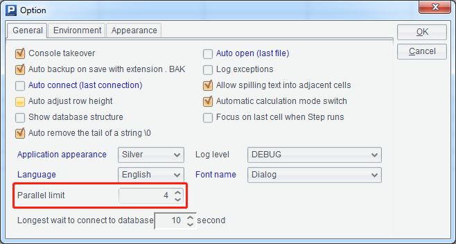
A1: List the name of the file which satisfies nid*T.ctx (here * is wildcard), and @p option means to return the file name with full path information. We also need to identify whether the parallel limit in the environment is set with a reasonable number when executing multi-thread using the fork function. Here 4 threads are used and the corresponding settings in the designer are as follows:

B1: Every thread creates the corresponding index file for each composite table and the final results are:

	A	B
1	=file("keys.txt").import@i()
2	=A1.group(~%N)
3	fork N.(~-1),A2	=A3(2)
4		=file("nid_"/A3(1)/"_T.ctx").open().icursor(;B3.contain(nid),nid_idx)
5		return B4
6	=A3.conjx()
7	=file("result_nid.txt").export@t(A6)

[Code 5.6]

 

The query procedures of Code 5.6 are explained in detail as follows:

 

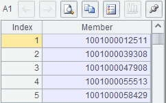
A1: Retrieve the sequence of query key values from keys.txt, and since the result is only one column, @i option is used to return the result as a sequence:

A2: Perform equivalence grouping on the sequence of A1 by the remainder by 4.

 

A3 and B3-B5: Use the fork function to parallel query each composite table by the equivalence-grouped key values. Here fork function is followed by two parameters, one is loop function N.(~-1), and the other is A2. In the following B3 and B4, use A3(2) and A3(1) to get the above-mentioned two parameters of the corresponding order respectively. B4 is to filter the data of the composite table file based on the key value set in B3. The cursor is returned in B5. Because there is a sequence of cursors returned by multiple threads in A3, we need to union all these cursors using the conjx function in A6.

 

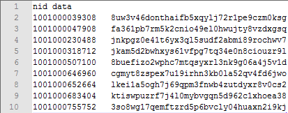
A6-A7: After union all the cursors returned by multiple threads, export the cursor records to the text file, and the first few lines are: