Big data usually requires external storage. To implement parallel computing in external storage, there must be better data segmentation technology, i.e., a technology that can easily divide the data into several parts so that each thread or process can process separately.

 

SPL adopts the double increment segmentation technology, which achieves the appendable blocking scheme on a single file, and has a particularly prominent advantage in parallel computing. In this article, we will analyze the principle of this technology in detail by simulating the process of writing data to a binary file, and will focus mainly on multi-thread cases, as the multi-process is similar.

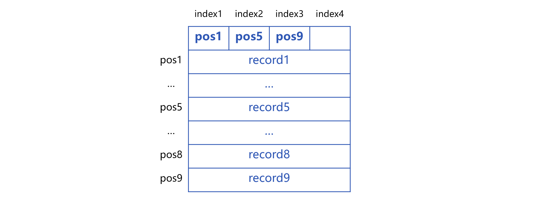
To implement the said technology, a fixed-length index area needs to be reserved at the header of binary file. For ease of understanding, we assume that the length N of index area is 4, which means that the index area has 4 index units index1 to index4. After the index area, write four consecutive records, the binary file looks like this:

In this figure, the section that stores the data is called the data area. The position of byte at the beginning of 4 records is represented by pos1 to pos4, and these positions will be written at the corresponding index unit of index area. The 4 pieces of data are physically continuous without any separator or blank area. Taking the positions pos1 to pos4 in these four units as the boundary, we can divide the data area into four parts, called four blocks, and each block contains 1 record, that is, the block capacity is 1.

In parallel computing, each block can be used as a segment, or multiple consecutive blocks can be combined into a segment. For example, when two threads are in parallel computing, two segments are required. The first segment starts at pos1 and ends at the byte before pos3; the second segment starts at pos3 and ends at the end of the file; each segment contains two consecutive blocks.

 

There is no empty position left in the index area before appending the 5th record to the data area. In this case, it needs to modify the index area first in a way that keep index1 unchanged, change the content of index2 to that of original index3, and clear index3 and index4. After modification, the original 4 blocks are merged into 2, and each block contains two records, and the capacity of block is doubled, we call this process double increment. The binary file will then look like this:

After double increment, append records 5 to 8, write pos5 into index3, and pos7 into index 4, after that, the file will become as follows:

At this time, there are 4 blocks in data area, and each block contains 2 records. We can see that during the data appending and double increment, the number, starting and ending positions and capacity of the blocks are changing, that is to say, the division of data area by the blocks is changing, therefore, it is a dynamic blocking.

 

When continuing to append the 9th record, there is once again no empty unit in the index area. We now need to modify the index area in the same way: keep index1 unchanged, change the content of index2 to that of previous index3, and clear index3 and index4. At this point, the second double increment is completed, as a result, the actual blocks are merged into 2, and each block contains 4 records, and the block capacity is doubled for the second time.

When appending the 9th record after the second double increment, write pos9 into index3. The data area now has 3 blocks, the first two contain 4 records respectively, and the last one has 1 record, like the figure below:

When appending more data, do the same thing as above. During this process, the number of records is increasing, and the fixed index area is modified continuously. However, the size of fixed index area remains unchanged, and the actual number of blocks is kept between 2 to 4. In addition, the number of records in each block is basically the same, except that the last block may have fewer records.

 

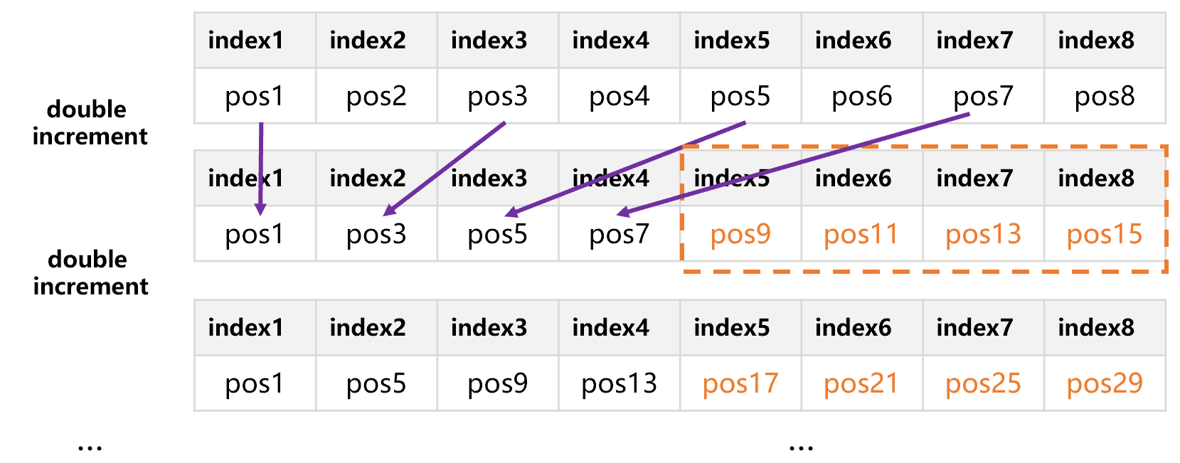
The actual number of blocks in the double increment segmentation scheme is between ½N and N, this number can be increased as long as the length N is increased. Suppose that we increase N to 8, since the data appending and double increment has same principle, it is easy to understand just by looking at the fixed index area, as shown in the figure below:

Now, the number of blocks is actually between 4 and 8, and it can support 4 to 8 parallel calculations at most. According to the number of CPU cores and concurrency capability of hard disks of mainstream computers, the number of parallel calculations is usually from several to dozens. If N is set to be larger like 1024, 2048, 4096, etc., we can divide the data into several to dozens of segments at will. But N should not be set too large, so as not to make the index area occupy too much space. SPL sets N to 1024, which is sufficient for mainstream computers.

 

In this way, the actual number of blocks is between 512 and 1024. Since these blocks are basically the same in size, after being combined into several to dozens of segments, the amount of segmented data to be processed by each thread will be very close to the average. In addition, since different threads of the same machine have basically the same computing power, it can ensure that the computing time of each thread is roughly the same in the end, hereby effectively avoiding the situation where some threads slow down the whole task.

 

In the double increment segmentation scheme, the data in the block are stored continuously. Therefore, using adjacent blocks to form segments can ensure that each thread reads the data continuously on the hard disk. In this way, it can avoid the performance of hard disk being greatly decreased due to frequent jumping reading.

 

In this scheme, the data can be appended continuously, and the index can be generated by double increment. For the new data generated in practice, just continue writing the data to the end of the file and perform the double increment in the same way. Since the index area is fixed in size, the modification of index area during double increment will not affect the stored data, and it does not need to take a lot of time to rebuild the entire file.

 

The aforementioned data are appended record by record, which belongs to the row-based storage. Since the double increment segmentation technology is based on the number of records, it is also particularly suitable for columnar storage. Columnar storage is essential to continuously store the same fields of every record. When adopting this technology, it needs to create its own fixed index area for each field. When the value of a certain field is written to the data area, it needs to write the starting position to the fixed index area of this field and perform the double increment as described above. Writing data to the index area of all fields and the double increment is performed synchronously, and are always consistent. This ensures that all fields are segmented synchronously, that is, the field at the beginning of a segment always belongs to the same record. For conventional columnar storage, it is difficult to achieve segmentation based on the number of records; generally, it will do the blocking first, and then implement the columnar storage inside the block, as a result, many blocks (to adapt to parallel computing) and large blocks (to adapt to columnar storage) are required, and it is only suitable for scenarios with a particularly large amount of data.

 

SPL’s composite table implements the double increment segmentation scheme, and can flexibly select the columnar storage or row-based storage based on actual scenario. The code is roughly as follows:

file("T-c.ctx").create(…).append(cs)

// Create the columnar storage composite table, and write the data from the cursor cs to the composite table.

file("T-r.ctx").create@r(…).append(cs)

// Create the row-based storage composite table, and write the data from the cursor cs to the composite table.

 

The code for parallel computing on composite table is also very simple. Let’s take the grouping and aggregating of multi-thread parallel computing as an example:

=file("T-r.ctx").open().cursor@m().groups(f1,f2,f3,…;sum(amt1),avg(amt2),max(amt3+amt4),…)

// Use the row-based storage when many columns are involved in the calculation, or when there are few columns in total.

=file("T-c.ctx").open().cursor@m(f1,amt1).groups(f1;sum(amt1))

// Use the columnar storage when there are many columns in total, but few columns are involved in the calculation.