

In-memory index of SPL
The index is similar to the “content” of the original table, which is a storage structure additionally created outside the original table. When searching and computing, we can first search the index to find the location of the original table in the “content”, and then go to the original table to find the corresponding record. The more fast the index query is than the original table query, the more obvious the speedup effect of the index query will be.
Index creation is a relatively independent process, which can be done in one go during the system initialization, and we only need to update the index regularly. In this article, we will introduce the in-memory index of SPL.
Position index
Sometimes, in order to perform the order-related calculations, we need to store the in-memory data table in an orderly manner by a certain field. In this case, if we also want to make the table ordered by other fields to optimize the performance, it will be in a dilemma.
For example, the order table contains the customer number field, time field and other fields, and the data are stored in chronological order, so that the time interval between two adjacent orders can be calculated conveniently. The calculation requirement we want to achieve is to search for the first order of the specified customer number, and then calculate the time difference between this order and the next adjacent order.
If we could find the position of the first record of the specified customer number in the order table, then we could calculate the time difference as long as we find the next record. However, since the order table is not ordered by customer number, we cannot use the binary search and can only use the sequential search, as a result, the search speed will be very slow. If the data is ordered by customer number, the position information in chronological order will be lost.
This problem can be solved by the position index algorithm provided by SPL. The first thing to do is to create a position index for the order table. For ease of understanding, we assume that the order table has only 10 records that are stored with position number (index) 1 to 10. The order data is ordered by the time field otime, and is out of order for the customer number cid, as shown in the leftmost orders table in Figure 1:
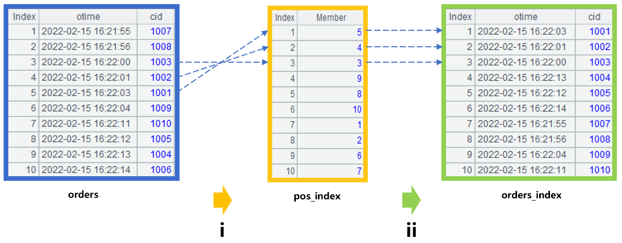
Figure 1: Creating position index
Step i in this figure is to create the position index pos_index, of which 10 members are ordered in ascending order by the customer number cid in the orders table, and the position number in orders table is index. For example, the first member of pos_index corresponds to the record with the smallest cid in orders table. Find the record with the smallest cid in orders table, and its index is 5, therefore, the value of the first member in pos_index is 5. In the same way, calculate the value of every member in pos_index, such as the value of second member value is 4...
Step ii is to create the sort table orders_index of orders. The members in sort table are determined in a way that first find the value of the same member in pos_index, and then take this value as the sequence number to obtain the corresponding record in orders table. For example: the value of the first member in pos_index is 5, then find the fifth record from orders, and take this record as the first member of orders_index. In this way, the generated orders_index is actually the result of orders sorted by customer number cid. It should be noted that orders_index does not copy the records of orders, but stores the address of the records, which can reduce the memory occupation.
Once the index is created, we can use it to implement query requirements. Assuming that the customer number cid to be queried is 1009, the calculation process can be illustrated by Figure 2 below:
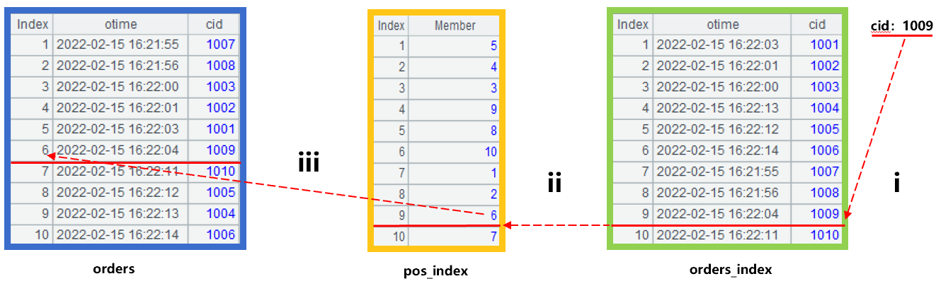
Figure 2: Search by position index
Step i is to use the binary search to search for the record with cid 1009 in the orders_index ordered by the customer number cid, obtaining its sequence number as 9. In step ii, find the member whose sequence number is also 9 in pos_index, obtaining its member value as 6, that is to say, 1009 corresponds to the sequence number 6 in orders. In step iii, find the record with sequence number 6 in orders, take its otime and the otime of the next record, to calculate the time difference, which is the result we need.
Step i uses the binary search, and step ii and iii use the position search. The overall complexity of the three steps is equivalent to that of binary search, and it is much faster than sequential search directly on orders.
SPL code that implements the above calculation is roughly as follows:
A |
B |
|
1 |
=file("orders.btx").import@b(otime,cid ) |
|
2 |
=A1.psort(cid) |
=A1(A2) |
3 |
=B2.pselect@b(cid:1009) |
=A1.calc(A2(A3),otime[1]-otime) |
A1: read the orders table ordered by otime.
A2: create the position index pos_index, corresponding to step i in Figure 1.
B2: create the sort table orders_index, corresponding to step ii in Figure 1.
A3: use the binary search to search for the position of the record with cid 1009, corresponding to step iii in Figure 2.
B3: A2(A3) corresponds to step ii in Figure 2, which is to find the position in the original table orders from the position index. Others correspond to step iii in Figure 2 to complete the calculation.
A1, A2 and B2 are the process of loading the data and creating the position index, and the results can be reused. This calculation process only needs to be performed once when the system is initialized and there is no need to do it every time during subsequent searches, hereby further improving the performance.
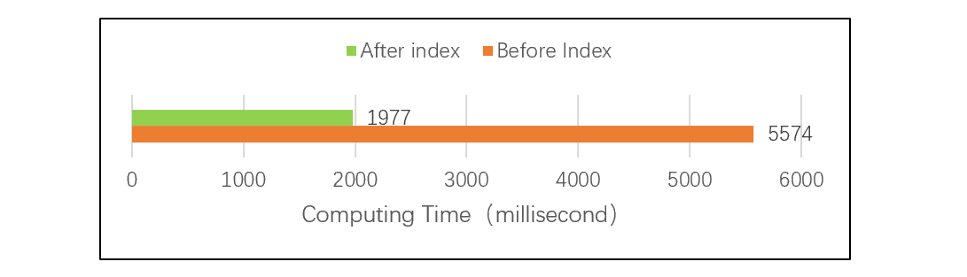
Actual test proves the advantage of position index in performance. Under the same amount of data and computing environment, the computing speed is increased by more than 80 times after using the position index. For details on the comparison test, visit: . The test results are as follows:
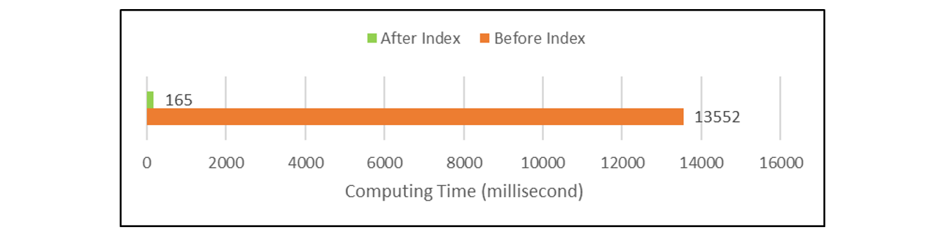
Test results figure 1: Position index comparison test
Hash index
Use a function to calculate the value of to-be-searched field (TBS field) to a natural number between 1 and M, which is called the hash value of the record, and this function is called the hash function. Having grouped the records of in-memory table according to the hash value, a two-layer structure H with length of M (where, there may be empty members) can be obtained, it is called hash index. The first layer of the hash index is the natural number between 1 and M, and the second layer is the subset consisting of original table records. Hash index does not copy the records in original table, but stores the addresses of corresponding records, which can reduce the memory occupation.
When searching for the specified value of the field, first calculate its hash value, and then locate the corresponding grouped subset in the hash index according to the sequence number, and finally use the sequential search or binary search in this grouped subset to find the target record.
For example, the user table contains fields such as id and user name (name), and we use the remainder method often used for integer field as a hash function of id. For ease of understanding, we assume that the user table has only 10 records, as shown in the leftmost users table in Figure 3:
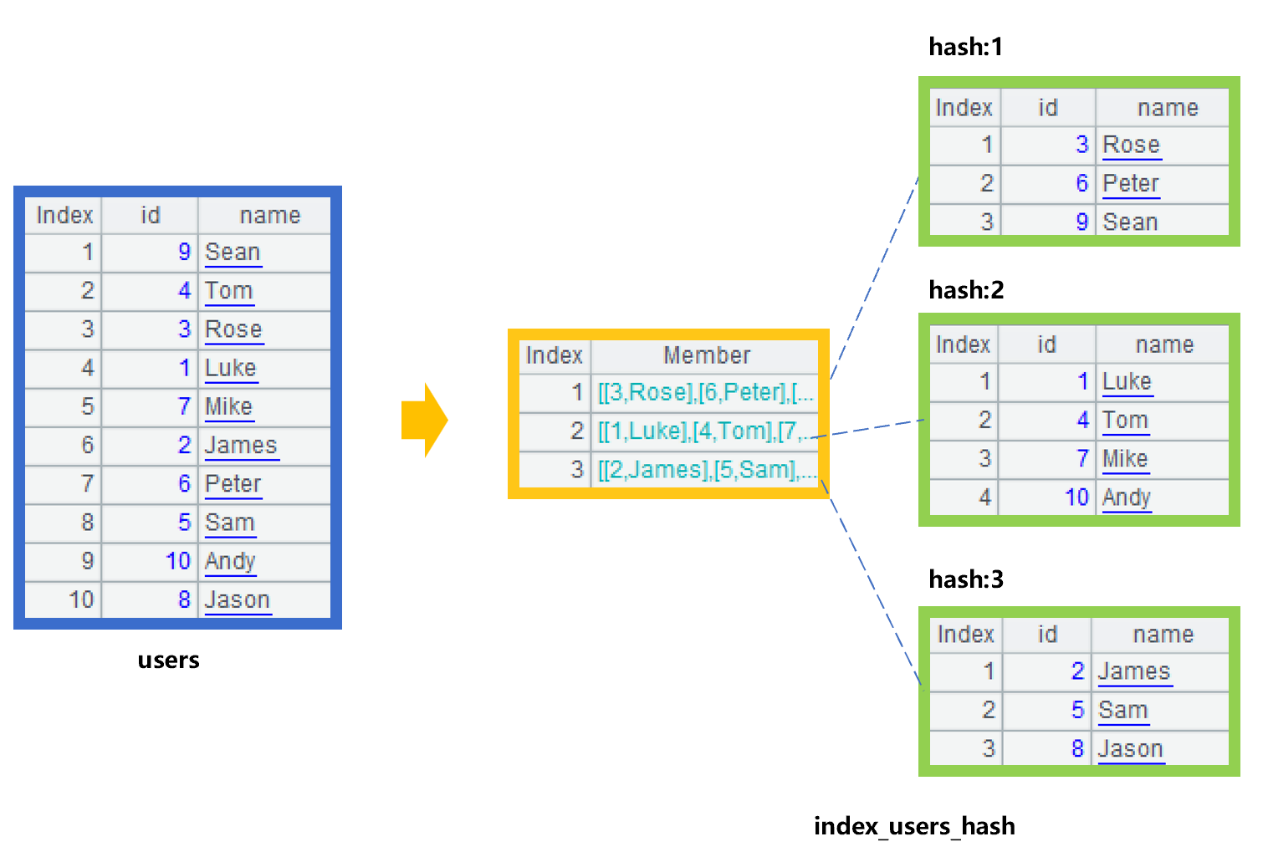
Figure 3: Creating hash index
First, calculate with id%3+1 on the values of id field of the users table to obtain the hash value of 1, 2 or 3, and then store the records into corresponding grouped subset according to the hash value of each record to generate the hash index. Since the data in these grouped subsets are ordered by id, we can use the binary search to speed up when searching within groups.
After the hash index is created, we can use it for searching the id field. Suppose we want to search for the user whose id is 7. See Figure 4 below for the general process:
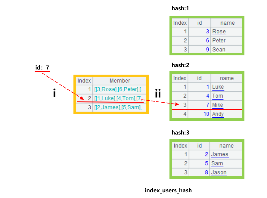 Figure 4: Search by hash index
Step i, first use the hash function to calculate the hash value of user whose id value is 7: 7%3+1 equals 2, and then determine the record to be searched is in the second grouped subset. Step ii, use the binary search to search for the record with cid 7 in the grouped subsets. If the data in the grouped subsets were not ordered by id, we would have to use the sequential search.
In this example, we divide 10 records into three groups. When searching, first locate according to the sequence number, and then perform the binary search. The amount of data to be searched in the grouped subset is only one third of the total amount of data. This example is lucky because the amount of data in the three groups of the hash index is relatively average. Of course, there are also unlucky situations, for example, when the remainder of most id values is 1 and 2, then the data amount in the three groups is very uneven.
Generally, let the total amount of data be N. When you are lucky, the amount of data in every grouped subset of hash index is close to N/M. Since the complexity of hash value calculation and sequence number position search is O(1), the search complexity after establishing hash index will be reduced by M times, which is equivalent to search an in-memory table with length of N/M. If you are unlucky, the number of members in each grouped subset of the hash index is very unevenly distributed, and the hash index search may not improve the performance in extreme cases, which depends on the design of the hash function and the distribution of the TBS key values in the original dataset.
However, luck is usually not too bad. In most cases, hash index will get better performance improvement, even has advantages over using sorting followed by binary search when the original data is out of order.
The disadvantage of hash index is that it needs to occupy memory space to store the index. If you want to speed up, you need a larger index and it will occupy more space.
SPL provides a hash index for the primary key, which will automatically use the system’s built-in hash function.
A |
B |
|
1 |
=file("users.btx").import@b(id,name ) |
|
2 |
=A1.keys@i(id) |
=A2.find(12345) |
3 |
=A1.keys@i(id;100) |
=A3.find(12345) |
In A2, when setting the primary key, we can use @i to create an index at the same time; In B2, if there is an index in place, the find() function will use it automatically; and in A3, when creating an index, we can also use parameters to control the length of the hash index (i.e., M value) to 100, and SPL programmer can adjust this length according to the actual situation.
Index reuse after filtering
In many cases, the in-memory data table may be filtered before performing other calculations such as association, grouping. If an index is already created for the data table, this index will not work after filtering. If an index is still required for further calculations, it has to be recreated. Creating an index, however, takes time because there is a need to calculate the hash value of primary key and so on. The time to create an index is not short when the number of records is still relatively large after filtering. Moreover, because the filtering condition is unpredictable, the index cannot be prepared in advance.
SPL provides a mechanism of reusing the index after filtering, which can directly delete the records in the index of original table that do not meet the filtering condition, in this way, the index can be reused after filtering.
Let’s take the hash index of the user table as an example. After filtering out the users whose name is neither Peter nor Tom, the process of index reuse can be roughly illustrated by Figure 5:
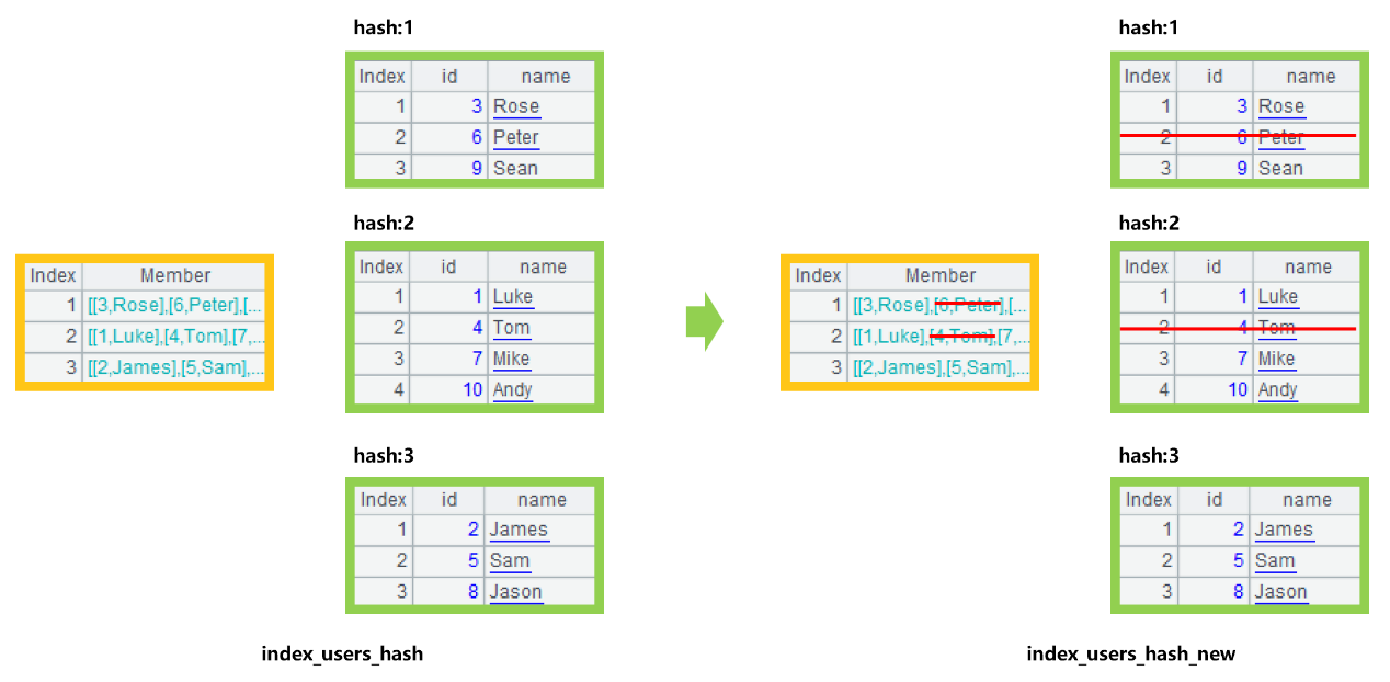
Figure 5 Index reuse after filtering
This figure shows that after deleting the records of Peter and Tom from the index of user table, a new index of the filtered result is directly generated, saving the time of creating a new index. However, we also found that if the number of filtered records is large (the remaining is small), the action for deleting the records in the index will not be very fast. Therefore, when the number of remaining records is smaller, recreating an index may be faster. Which method to use depends on the actual situation.
SPL code for index reuse after filtering is roughly written as follows:
A |
|
1 |
=file("users.btx").import@b(id,name ).keys@i(id) |
2 |
=A1.select@i(name!="Peter" && name!="Tom") |
3 |
=A2.find(9) |
In A2, select@i uses the mechanism of reusing the index after filtering, and the filtered result has a primary key index.
When searching for the primary key in A3, the new index is used.
Multi-layer sequence number index
SPL provides the sequence number positioning algorithm, which is described in detail at: , and we just give a brief introduction here. If the value of TBS field is exactly the same as the position of the record in the in-memory data table, we can use the specified field value to directly take the record at the corresponding position in data table.
For example: the id field of user is a continuous natural number starting from 1, and the data are stored in the in-memory user table in order by id. If we want to search for the user whose id is 12345, we can directly take the record whose position is 12345 from the user table. When the sequence number positioning is used, no comparison is required, and its search complexity is O(1); moreover, there is no need to create an index outside the original table.
However, in some cases, the sequence number positioning is not applicable. For example, the ID number of the Chinese citizen is made up of a series of numbers, which can be understood as a natural number, and is naturally a sequence number, but we cannot search for the ID numbers by aligning them to the natural number, and then using the sequence number positioning.
The reason is that the sequence number positioning requires a sequence of not less than the largest sequence number to store all the records to be searched and the null values to fill in the vacancy. If the ID number is converted directly into a natural number, the sequence number range will be too large to be held in the current computer memory (1017, the ID number has 18 digits, ignoring the last check digit), as a result, the number of sequence numbers to be filled with null is much more than the number of sequence numbers with records. In this case, the sequence number positioning cannot be directly used.
To solve this problem, SPL provides the multi-layer sequence number positioning and serial byte index algorithms. Let's take an example of searching for people by ID number, and we will use the common characteristics of the people to be searched to make the ID numbers distribution relatively centralized, instead of covering the range of all 18-digit natural numbers. Using this characteristic, a multi-layer sequence number positioning can be constructed to reduce the space occupied in the implementation of sequence number positioning.
For example, for the people born in Beijing between 2016 and 2018, since both the birth dates and region are relatively centralized, we can create a three-layer sequence number index as shown in Figure 6 below:
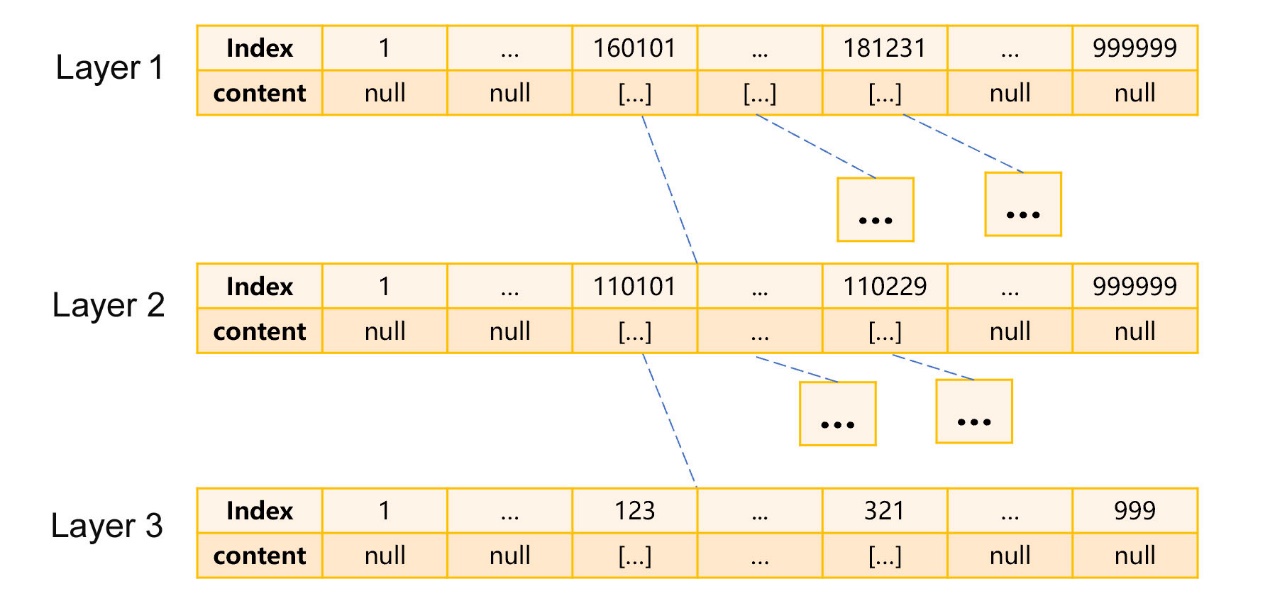
Figure 6: Creating multi-layer index
The first layer is the date of birth. We only need to focus on the last two digits because there will be no repetition. Therefore, we can regard the date of birth as a continuous natural number with a maximum value of 999999, which means that the ID numbers are divided into 999999 grouped subsets according to the date of birth. For example, the ID number on January 1, 2016 is assigned to the group at the position of 160101. Since there are about 1000 dates from 2016 to 2018, the first layer has only 1000 non-null members, and the rest are null.
The second layer is the region. In this layer, the ID numbers of each date are divided into 999999 grouped subsets according to the first 6 digits (region number). For the member that is null in the first layer, it is still null in the second layer, that is, the total number of members in the second layer is about 1000*999999. There are only about 20 regions in Beijing, and hence there are about 1000*20 non-null members in the second layer.
The third layer is the last 3 digits of the ID number (excluding the check digit). According to the number of non-null members in the first and second layers, there are about 1000*20*999 members in this layer.
In this way, the total number of members in the three layers is: 999999+1000*999999+1000*20*999, equaling about 1G, and occupying the space of a few G or a dozen G, which can be held in modern computers.
It can be seen from Figure 6 that SPL takes the multi-layer index as a tree structure. If the data meets the above-mentioned characteristics of concentrated distribution, it seems that most branches of the tree will not extend to the deepest layer, but will break at the shallower layer, therefore, it will no longer occupy the space. The space occupied by the whole tree may be so small that the memory can hold.
Multi-layer sequence number positioning can only be used when there are many null values in the first few layers after layering. If there are few or no null values, the space occupied by multi-layer sequence number structure is larger than that of single layer.
Once the multi-layer index is created, we can use it to query the specified ID number. For example, to query 110101201601013212, the process is roughly as shown in Figure 7:
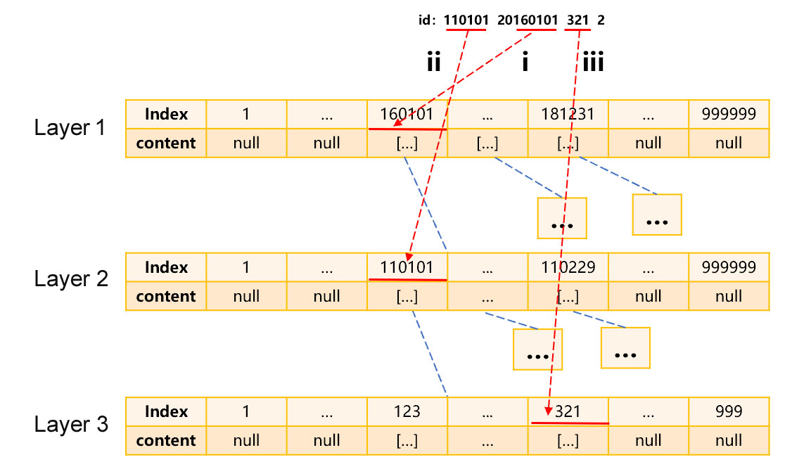
Figure 7: Search for ID number by multi-layer position index
Step i, use the last 6 digits of the birth date, i.e., 160101, to find the first-layer grouped subset at the position of 160101 in the first-layer index; Step ii, in this grouped subset, use the first 6 digits of the ID number, i.e., 110101, to find the second-layer grouped subset at this position; Step iii, still in this grouped subset, use the last 3 digits of the ID number, i.e., 321 (excluding the check digit) to find the third-layer grouped subset; and finally, search for the ID number in the third-layer grouped subset.
The use conditions of multi-layer sequence numbers are relatively complex. When there are many layers or the operation of generating a serial byte is complex, sometimes it is not more advantageous than ordinary hash index.
SPL provides a data type specifically for multi-layer sequence number index, called serial byte, which consists of two long, and each byte of two long represents a layer, and thus the sequence number range of each layer is 0-255, and can support up to 16 layers of sequence numbers.
For example, when we want to convert an ID number without the check digit to a serial byte, we must ensure that each layer is within 0-255. In this case, we can take the digits according to the ID number from left to right directly, two digits at a time. The value of the birthday year -1900 is also less than 255, which can be used as a layer. The conversion relationship between the ID number 110101201601013212 and the serial byte is shown in Figure 8:

Figure 8: Conversion relationship between ID number and serial byte
Since there are only 8 layers, only one of the two long of the serial byte k is used, and its value is b01017401012001. The first hexadecimal value b corresponds to the first two digits of the ID number, i.e., 11, and the rest two digits are taken in a similar way. Only the year is special, which uses 2016-1900=116, converting to hexadecimal value, that is 74.
This example takes the digits directly from left to right according to the ID number, which is not necessarily the most suitable in the actual scene. In practice, we should to adjust the order of layers in the serial byte according to the known data distribution characteristics.
SPL code for creating a multi-layer position index with the serial byte is roughly as follows:
A |
B |
|
1 |
func |
return k(int(left(A1,2)),int(mid(A1,3,2)),int(mid(A1,5,2)),int(mid(A1,7,4))-1900,int(mid(A1,11,2)),int(mid(A1,13,2)),int(mid(A1,15,2),int(mid(A1,17,1)) |
2 |
=T.run(id=func(A1,id)).keys@is(ID) |
|
3 |
'110101201601013212 |
|
4 |
=A2.find(func(A1,A3)) |
|
A1 defines a function that can convert the ID number to a serial byte as shown in Figure 8.
A2 converts the ID number in the table to a serial key, and then creates an index using @s, that is, to construct the above-mentioned tree structure.
A4 uses the serial byte index to search for the ID number.
Actual test shows that under the same amount of data and computing environment, the computing speed is increased by nearly three times after using the serial key index. For details on the comparison test, visit: , and the test results are as follows:
Test results figure 2: Serial byte index comparison test
SPL Official Website 👉 https://www.scudata.com
SPL Feedback and Help 👉 https://www.reddit.com/r/esProcSPL
SPL Learning Material 👉 https://c.scudata.com
SPL Source Code and Package 👉 https://github.com/SPLWare/esProc
Discord 👉 https://discord.gg/cFTcUNs7
Youtube 👉 https://www.youtube.com/@esProc_SPL


Chinese version