Least-squares algorithm linear fitting
The steps of least squares fitting are:
Given a set of data points(x1,y1),(x2,y2)……(xm,ym)
(1)Determine the type of curve to be used to fit the data, for example 
(2)Substitute the data points into the curve and get the system AX=Y
(3)Solve AX=Y using linefit() linear least square method
For example, the data in the following table is fitted with the least square method
x |
19 |
25 |
31 |
38 |
44 |
y |
19 |
32.3 |
49 |
73.3 |
97.8 |
SPL code:
A |
|
1 |
[19,25,31,38,44] |
2 |
[19,32.3,49,73.3,97.8] |
3 |
=canvas() |
=A3.plot("NumericAxis","name":"x") |
|
5 |
=A3.plot("NumericAxis","name":"y","location":2) |
6 |
=A3.plot("Dot","lineWeight":0,"lineColor":-16776961,"markerWeight":1,"axis1":"x","data1":A1,"axis2":"y","data2": A2) |
7 |
=A3.draw(800,400) |
8 |
[[19,1],[25,1],[31,1],[38,1],[44,1]] |
9 |
=linefit(A8,A2).conj() |
10 |
=to(10,50) |
11 |
=A10.([~,A9(1)*~+A9(2)]) |
12 |
=A3.plot("Line","markerStyle":0,"axis1":"x","data1":A11.(~(1)),"axis2":"y", "data2":A11.(~(2))) |
13 |
=A3.draw(800,400) |
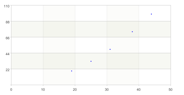
A1-A7 Import the data, draw the scatter plot, and determine the curve type
A3 Generate canvas
A4 Draw horizontal axis "x"
A5 Draw the vertical axis "y"
A6 Plot point primitives. The X-axis data is A1, and the Y-axis data is A2
A7 The distribution of observation points is linear, and the type of fitting curve is selected as
A8-A9 Take the data points into the curve and write them in matrix form, get
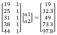 , as the AX=Y form
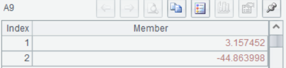
Pass the matrix parameters into linefit(A,Y) and the value of a1, a2 are solved, a1 =3.157452,a2=-44.8639981
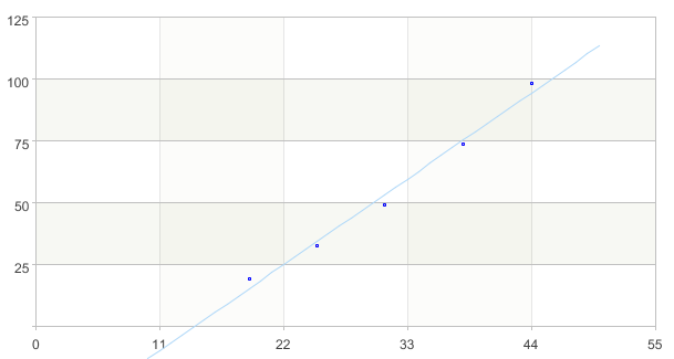
A10-A13 Draw the fitted curve onto the scatter plot for intuitive comparison
There are many types of curves that can be fitted using linear least square method linefit(). Common ones are:
(1) Line
(2) Polynomial 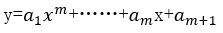
(3) Hyperbola 
(4) Exponential curve 
For hyperbolic and exponential curves, variable substitution is required to transform them into linear functions of a1 and a2
SPL Official Website 👉 https://www.scudata.com
SPL Feedback and Help 👉 https://www.reddit.com/r/esProcSPL
SPL Learning Material 👉 https://c.scudata.com
SPL Source Code and Package 👉 https://github.com/SPLWare/esProc
Discord 👉 https://discord.gg/2bkGwqTj
Youtube 👉 https://www.youtube.com/@esProc_SPL