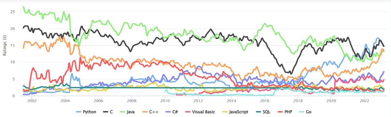
Quantitative trading involves using probability theory, statistical and other knowledges through programming and modeling to analyze massive amount of historical data, identify patterns and develop quantitative models, and then relying on computers’ powerful computing capabilities to make trading decisions fast and efficiently. There are many programming languages to choose from. The chart below is from the TIOBE index, showing the top 10 programming languages from 2002 to the present. It can be seen that, for a long period, Java and C dominated the rankings, but since 2018, with the rise of artificial intelligence, Python’s status has risen rapidly and now surpasses Java and C.

The same thing happens in the quantitative research field. The mainstream languages used to be Java, C, C++, R and Matlab, but now Python is predominantly used. Indeed, compared to languages like Java and C, Python is simpler to program, offers a rich collection of mathematical and statistical functions, and is very convenient to use.

However, often SPL is even more convenient to use for developing quantitative models. SPL boasts interactive programming, powerful data preparation capabilities, and flexible structured data processing methods to name a few. Although the language’s mathematical functions are not as extensive as Python’s, but advanced mathematical functions and large AI models are rarely used in quantitative analysis, where the commonly used algorithms are mostly linear models, data smoothing, PCA, statistical tests, etc. And all of them are available in SPL. For machine learning, SPL can encapsulate Python’s functionalities to achieve automated modeling. This is more convenient even than using Python directly.

An example will talk more and give the firsthand experience.

1. Classic strategy: Implementation and backtesting of dual moving average crossover strategy

The dual moving average crossover strategy uses two moving averages – one is the long-term moving average (such as a 10-day MA) and the other is the short-term moving average (such as a 5-day MA) – to predict the future trend of stock prices. The strategy is based on the assumption that stock price momentum moves toward the short-term moving average. When the short-term moving average crosses above the long-term moving average, it indicates upward momentum, suggesting a potential rise in stock price. When the short-term moving average crosses below the long-term moving average, it indicates downward momentum, suggesting a potential decline in stock price.

According to this pattern, let’s design a dual moving average crossover trading strategy using data of stock whose code is “002805”, and backtest it using the stock data in the year 2021. The initial capital is ¥50,000, and the transaction fee rate is 0.0003.

The strategy design consists of two parts – strategy writing and backtesting. The backtesting indicator is a single year’s yield. Here are the steps:

Write the strategy:

(1) Import data, sort them by date in ascending order, and select data of the year 2021;

(2) Compute 5-day MA and 10-day MA, and add results to the data;

(3) Set a transaction signal (named signal). When 5-day MA is greater than 10-day MA, record it as 1; otherwise, record it as 0;

(4) Place orders according to changes of the signal value. When signal changes from 0 to 1, buy the stock; and when it changes from 1 to 0, sell it. The position size in each transaction are 1,000 shares. And use order field to record order amount in each transaction.

Backtest the strategy:

(1) Use stock field to represent the stock position. Its value is the sum of all existing position sizes (order total).

(2) Use stock_value to represent the stock market price, which is equal to position size*stock price.

(3) Use acctrade_cash to represent the total transaction amount, which includes order amount and transaction fee.

(4) Use available_cash to represent the available cash, which is initial capital – cumulative transaction amount.

(5) Use total to represent the total capital, which is available cash + stock market price. The change of total capital is the yield.

Now we use Python and SPL respectively to write and backtest the strategy:

Python code:

import pandas as pd
import numpy as np
pd.set_option("display.max_rows",None)
pd.set_option("display.max_columns",None)
initial_cash=50000
fee=0.0003
# Dual moving average crossover strategy
data = pd.read_csv("D://002805.csv", encoding='gbk')

data["Date"]=pd.to_datetime(data["Date"])

data = data.sort_values("Date")

data = data.loc[(data["Date"]>"2021/01/01")& (data["Date"]<"2022/01/01")]


data["MA_5"]=data["Close"].rolling(5).mean()
data["MA_10"]=data["Close"].rolling(10).mean()
data["signal"]=np.where(data["MA_5"]>data["MA_10"],1,0)
data["order"]=data["signal"].diff()*1000
#Backtesing
position = pd.DataFrame(index=data.index).fillna(0)
position["Date"]=data["Date"]
position["stock"]=data["order"].cumsum()
position["stock_value"]=position["stock"]*data["Close"]
position["acctrade_cash"]=(data["order"]*data["Close"]*(1+fee)).cumsum()
position["avaiiable_cash"]=initial_cash-position["acctrade_cash"]
position["total"]=position["available_cash"]+position["stock_value"]
#Investment income
returns=(position["total"].iloc[-1]-initial_cash)*100/initial_cash
print(returns)

SPL code:

	A	B
1	>initial_cash=50000
2	>fee=0.0003
3	=T(“D://002805.csv”).sort(Date).select(Date>date(“2021/01/01”) && Date<date(“2022/01/01”) )
4	=A3.derive(Close [-4:0]:Close_5,avg(Close [-4:0]):MA_5,avg(Close [-9:0]):MA_10,if(MA_5>MA_10,1,0):signal,(signal-signal[-1])*1000:order)	Strategy
5	=A4.new(stock[-1]+order:stock,stockClose:stock_value,acctrade_cash[-1]+orderClose*(1+fee):acctrade_cash)	Backtesting
6	=A5.derive(initial_cash-acctrade_cash:avaliable_cash,avaliable_cash+stock_value:total)

Compare the Python code and the SPL code and we find the following differences:

(1) In terms of the code amount, Python involves over 20 lines while SPL only has several lines.

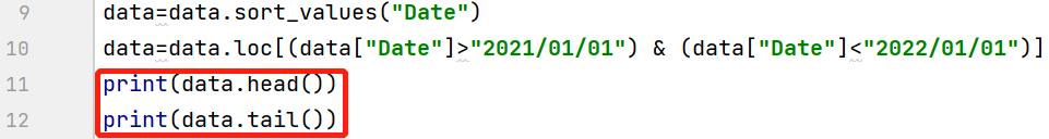
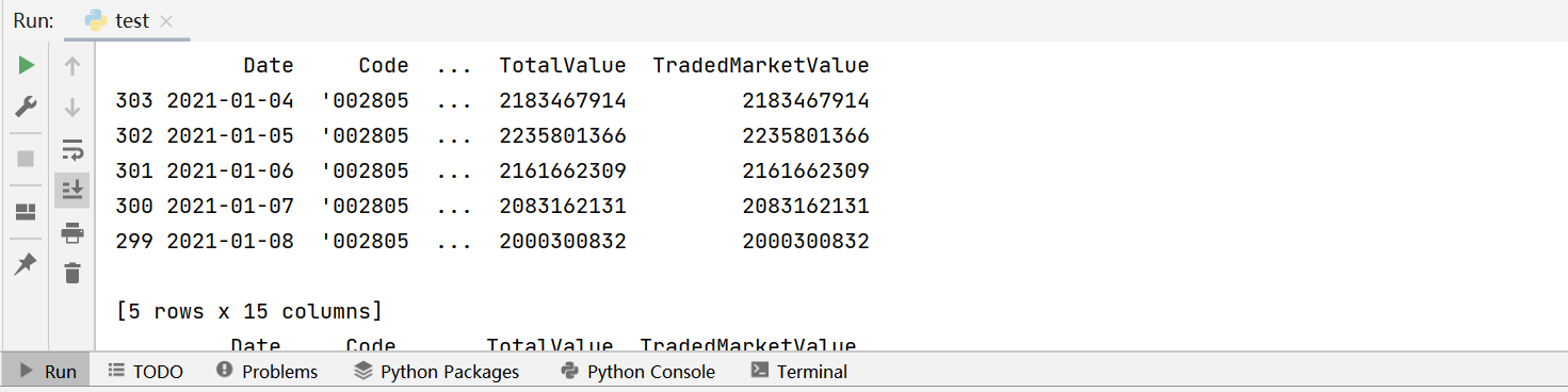
(2) Quantitative programming is highly experimental, and on many occasions requires real-time monitoring of the results. Though there are many IDEs available for Python programming, such as Pycharm, Eclipse and Jupyter Notebook, the most frequently used method is still using print()to print target values to view. To check whether the result of selecting and sorting data of the year 2021 is correct, for example, we need to use print() function after the corresponding Python statement, as shown below:

The code returns the following result:

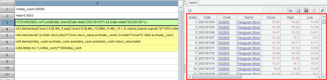
SPL uses interactive programming technique. The result of executing each line of code is directly displayed on the interface, without the need of specially printing it out. Besides, the display mode is like an Excel table, which is very user-friendly.

(3) Python adds fields one by one and repeatedly references the table, while SPL derives or creates multiple fields directly and just references the table once. The SPL code is simpler and more efficient.

(4) SPL directly references a neighboring record to compute, creating more intuitive code. Python cannot implement the direct reference of a neighboring record, and needs to achieve the same functionality through the other functions. Take the computation of moving average as an example:

Compute moving average in Python:

data["MA_5"]=data["Close"].rolling(5).mean()
data["MA_10"]=data["Close"].rolling(10).mean()

Compute moving average in SPL:

A3.derive(Close [-4:0]:Close_5,avg(Close [-4:0]):MA_5,avg(Close [-9:0]):MA_10)

SPL uses the form of Close[-4:0] to reference closing prices of neighboring 5 days and computes their average. Python uses the rolling()function to compute average. It appears that both statements are concise. But when we check Pandas’ rolling() method, we find it returns a subobject instead of the neighboring 5-day closing prices. Similar to groupby()method, it generally works with an aggregate function, such as mean() or sum(). In an ordinary data analytics scenario, a simple average or summary method is enough. But for the quantitative computing, that’s far from enough. For example, if we want to make the 5-day moving average price indicator more responsive, we compute weighted average according to the varying degrees of importance 5:4:3:2:1. Then we look up the function reference document, which shows that, by default, every window value has the same degree of importance but there are the other ways of distribution of degrees of importance, and that more is explained in related SciPy document. As of now, Python’s implementation becomes complicated and difficult to learn.

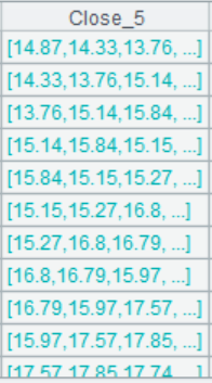
It is much simpler to make the modification in SPL because “Close[-4:0]” returns the 5-day closing prices (as shown below), which can be directly referenced for the computation. Below also shows the corresponding code:

	A
1	=[5,4,3,2,1]
2	=A1.sum()
3	=T(“D://002805.csv”).sort(Date).select(Date>date(“2021-01-01”) && Date<date(“2022-01-01”) )
4	=A3.derive(Close[-4:0].sum(~*A1(#)/A2):WMA)

“~” and “#” are used in a loop function to get the current value and its sequence number respectively.

2. Computing RSI indicator

Let’s look at a bit more complicated example – computing RSI indicator.

Relative Strength Index, RSI is a momentum indicator developed by Welles Wilder and commonly used for technical analysis of short-term and medium-term stock trading.

RSI is a type of technical curve plotted according to percentages of total stock price increase to the total stock price change during a certain period. The curve displays the relative strengths and weaknesses during the past N days, which reflect the market situation in the given period.

The range of RSI values is from 0 to 100. The larger the value, the better the stocks perform. Most of the time RSI values fluctuate between 30 and 70. Stocks with RSI > 80 are considered overbought, and it is more likely that a decrease in price will happen; and with RSI < 20, stocks are considered oversell, and it is more likely that an increase in prices will occur.

Method of computing RSI:

RSI = (N-day price increase SMA / N-day price increase/decrease SMA)*100%

SMA represents simple moving average.

SMA=1-day price increase/N+(1-1/N)*SMA of the last trading day

1-day price increase = closing price – closing price in the last trading day

Take the positive value of the 1-day price increase within N days

Take the absolute value of the 1-day price increase/decrease within N days

Let’s implement the computation in Python and SPL respectively:

“Change” field is the 1-day price increase

“sma_up_change” field is the increase SMA

“sma_abs_change” field is the increase/decrease SMA

Python code:

import datetime
import pandas as pd
import numpy as np
pd.set_option("display.max_rows",None)
pd.set_option("display.max_columns",None)
n = 14
data=pd.read_csv("D://002805.csv", encoding='gbk')
data["Date"]=pd.to_datetime(data["Date"])
data=data.sort_values("Date")
data=data.loc[(data["Date"]>"2021/01/01")& (data["Date"]<"2022/01/01")]
data["Change"]= data["Close"]-data["Close"].shift(1)
data["Change"].iloc[0]=data["Close"].iloc[0]
length=len(data)
sma_up_change =[0]*length
sma_abs_change = [0]*length
rsi = [0]*length
sma_up_change[0]=data["Change"].iloc[0]/n
sma_abs_change[0]=sma_up_change[0]
for i in range(1,length):
    sma_up_change[i]=max(data["Change"].iloc[i],0)/n+(1-1/n)*sma_up_change[i-1]
    sma_abs_change[i]=abs(data["Change"].iloc[i])/n+(1-1/n)*sma_abs_change[i-1]
    rsi[i]=sma_up_change[i]/sma_abs_change[i]*100
data["rsi"]=pd.Series(rsi,index=data.index)

SPL code:

	A
1	14
2	=T(“D://002805.csv”).sort(Date).select(Date>date(“2021/01/01”) && Date<date(“2022/01/01”) )
3	=A2.new(Date,Close-Close[-1]:Change)
4	=A3.derive(max(Change,0)/A1+(1-1/A1)*sma_up_change[-1]:sma_up_change,abs(Change)/A1+(1-1/A1)*sma_abs_change[-1]:sma_abs_change)
5	=A4.new(Date,sma_up_change/sma_abs_change*100:RSI)

Python involves over 20 lines of code, while SPL only needs several lines.

There are two differences in their implementations:

(1) Different methods of referencing the closing price in the previous day when computing 1-day price increase = closing price – closing price in the last trading day.

Python：

data["Close"].shift(1)

SPL:

Close[-1]

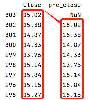
Python uses the offset matrix indexing method, where closing prices are shifted down by one row, as shown in the figure below. This illustrates the concept of a DataFrame as a “frame” of data, which does not allow direct reference of neighboring rows. Users can only use an alternative method to work around this limitation. Also, this method to reference a neighboring row is completely different from the method in the previous example for getting multiple neighboring rows. In other words, just because you know how to reference one row doesn’t mean you know how to reference multiple rows, and even if you know how to reference multiple rows, you may not know how to do so using different methods (such as MA, WMA). In terms of learning methodology, Python doesn’t naturally lend itself to learn and apply by analogy. Therefore, while Python may seem easy to get started with, mastering it is not as easy - it feels like the more you learn, the more there is to learn.

SPL’s advantages are obvious in this regard, as it allows directly retrieving neighboring records using expressions like [-1] or [-4:0]. The way formulas are written is similar to other quantitative trading software. It follows the natural logic that is easy to understand. Once you have mastered the basic syntax, you can easily apply the experience to the other scenarios without memorizing too many functions.

(1) When calculating the SMA, Python does not support performing loop computations directly within a DataFrame. We need to extract the data, compute it with “for” loop, and then place it back into the DataFrame. However, SPL allows referencing each row of data directly and performing recursive computations directly on the table sequence, c creating smooth and easy coding process.

The quantitative computing involves frequent references of neighboring records, and the Python implementation is a hassle.

Python:

length=len(data)
sma_up_change =[0]*length
sma_abs_change = [0]*length
rsi = [0]*length
sma_up_change[0]=data["Change"].iloc[0]/n
sma_abs_change[0]=sma_up_change[0]
for i in range(1,length):
    sma_up_change[i]=max(data["Change"].iloc[i],0)/n+(1-1/n)*sma_up_change[i-1]
    sma_abs_change[i]=abs(data["Change"].iloc[i])/n+(1-1/n)*sma_abs_change[i-1]
    rsi[i]=sma_up_change[i]/sma_abs_change[i]*100
data["rsi"]=pd.Series(rsi,index=data.index)

SPL:

	A
…	…
4	=A3.derive(max(Change,0)/A1+(1-1/A1)*sma_up_change[-1]:sma_up_change,abs(Change)/A1+(1-1/A1)*sma_abs_change[-1]:sma_abs_change)
5	=A4.new(Date,sma_up_change/sma_abs_change*100:RSI)

It can be seen from these two examples that the quantitative computing largely involves various operations of structured data, especially those on neighboring rows. However, Python’s handling of structured data is not flexible, often requiring workarounds. Moreover, each type of operation requires a different method. Writing programs in Python can be mentally taxing, and learning the language is relatively difficult.

SPL is more flexible in both field and row record manipulations. SPL coding more aligns with natural logic. Algorithms expressed in formulas are clear and straightforward. Additionally, the way formulas are written is similar to that in the other quantitative trading software, making them easy to understand. The learning curve for SPL is also relatively smooth – once we master the basic syntax, we can flexibly manipulate structured data without the need to learn various libraries and functions.

A deep comparison between Python and SPL is discussed in Comparison between SPL and Python in processing structured data.

Not only is SPL simpler to code and has a flatter learning curve, but in most cases, it also computes faster. It makes it easier to implement parallel processing and handle larger datasets. All of these are explained in detail in the cited article.

Python’s computational ability is somewhat weaker, but its strength lies in the large number of libraries, such as Ta-Lib, which includes a variety of technical market indicators. This makes it very easy for beginners to get started. However, to build a good quantitative model and develop unique strategies, it is essential to understand the basic algorithms, as performing the computations yourself is the most reliable approach.