In many business scenarios, there is a phenomenon of data imbalance. For example, the defaulters in bank loan account for only a small portion of the borrowers; the fraudsters in insurance are individual phenomena; the proportion of defective products to all products is small; the unscheduled shutdown phenomenon in industrial production occurs rarely, and so on. All of these rare phenomena occur at a very low rate. But once they occur, large losses will result. In this article, we will talk about how to use YModel to predict the occurrence of these phenomena.

1. Prepare historical data

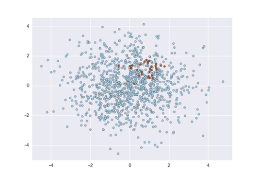
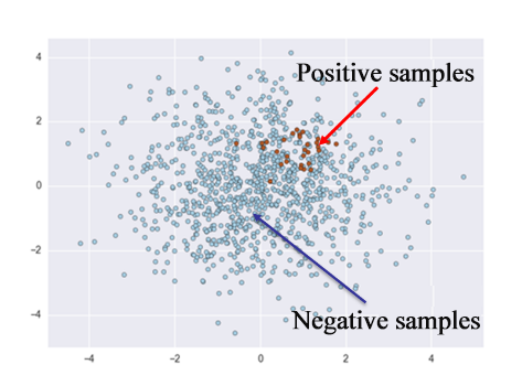
In historical data, the records where the rare phenomena have occurred are called positive samples, and the rest are called negative samples. Data imbalance means that positive samples are too few. For example, there are only a dozen positive samples in a dataset of tens of thousands. In this case, even though the total amount of data is large, it is difficult to build an effective model. Therefore, when preparing data, it is necessary to extract as many positive samples as possible. There is no fixed requirement on the specific number of positive samples. In general, the more complex the problem, the more the number of positive samples required. However, even a simple problem usually requires at least a few hundred positive samples to build a usable model. On the other hand, we can not extract only positive samples. For example, if we want to build a model to predict the default of loan customers, in addition to ensuring that the data of defaulting customers reaches a certain number, we also need to collect the data of normal customers.

2. Build the model

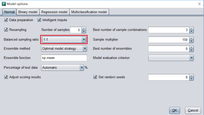
Import the prepared data into YModel, and then just perform automatic modeling. For unbalanced data sets, YModel can automatically sample to balance the ratio of positive samples to negative samples, so users do not need to operate themselves. However, we can modify and set the required Balanced sampling ratio ourselves, as shown in the figure. For beginners, it is usually recommended to adopt the default ratio.

3. Predict

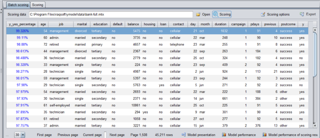
After building the model, perform prediction and get the prediction results. Similarly, sort the predicted probability results from high to low. After that, we just need to find the top-ranked customers or samples for targeted investigation, because rare phenomenon is more likely to occur in them.

4. Recall rate

In scenarios where data distribution is imbalanced, it is meaningless to focus solely on accuracy. A more meaningful indicator is the recall rate.

Recall ratio represents the proportion of correctly predicted positive samples among all positive samples.

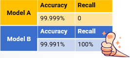
Let’s take an exaggerated example. An airport wants to build model to identify terrorists. Obviously, terrorists are an extremely small minority and represent a rare phenomenon. Suppose there are five terrorists among one million people. If we use accuracy to evaluate model, then as long as we identify all people as normal people, the accuracy of the model can reach as high as 99.999%, such as model A. However, it is clear that such a model doesn’t make any sense, as it does not identify any terrorist. Now let’s see model B, although its accuracy is somewhat low, the recall ratio is very high. It can identify all terrorists. While it is possible to misidentify a few normal people as terrorists, it is much better than missing the terrorists. Therefore, model B makes sense.

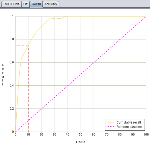
In YModel, we can use the recall curve to determine the recall rate. As shown in the figure below, the abscissa represents the percentage of the predicted rare phenomena occurrence probabilities sorted from high to low, with 10, 20... representing the top 10%, 20%... of samples respectively. The ordinate represents the recall value corresponding to each ranking stage. For example, the recall rate corresponding to 10 on the abscissa in the figure is about 0.75, indicating that 75% of the rare phenomena can be captured from the data ranked in the top 10% of the predicted probability results. In other words, compared with screening all the samples, 75% of rare (abnormal) cases can be found with 10% of the workload. The closer the recall curve is to the upper left corner, the stronger the ability of the model to capture rare phenomena such as default, fraud, defective products, abnormal equipment.