Data Analysis Programming from SQL to SPL: Access Duration
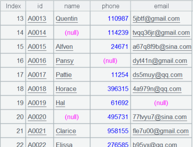
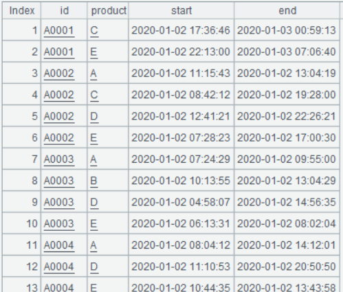
The following is part of the data from the simplified account table ‘user’ and access table ‘view’:
user:
view:
1. Calculate the number of minutes each account spent accessing each product
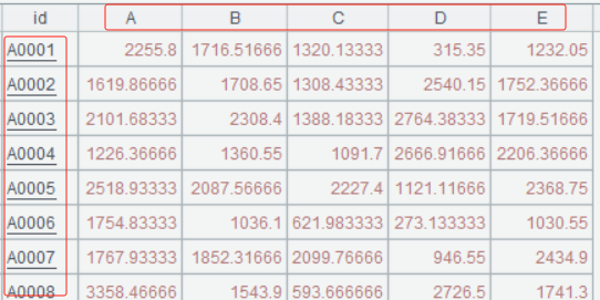
Group by account id and product, and then aggregate the number of minutes of each group. The results contain the columns account id, product and number of minutes. We want to pivot the results to the following format: account id, product A minutes, product B minutes, product C minutes, and so on.
SQL code:
select id,
  sum(if(product='A',timestampdiff(minute,start,end),0)) A,
  sum(if(product='B',timestampdiff(minute,start,end),0)) B,
  sum(if(product='C',timestampdiff(minute,start,end),0)) C,
  sum(if(product='D',timestampdiff(minute,start,end),0)) D,
  sum(if(product='E',timestampdiff(minute,start,end),0)) E
from view
group by id;
In SQL, you need to define separate aggregations for each product. Since there are 5 products, you’ll have to write the aggregation expression 5 times.
Oracle provides the pivot function:
select *
from (
  select
    id, product,
    (extract(day from (end - start)) * 24 * 60 +
     extract (hour from (end - start)) * 60 +
     extract (minute from (end - start))) AS minute
  from view
)
pivot (
  sum(minute)
  for product IN ('A', 'B', 'C', 'D', 'E')
)
Since Oracle doesn’t have the timestampdiff function, calculating the duration between two dates is relatively cumbersome.
While the pivot function is available, coding isn’t simple because column names cannot be omitted. Moreover, even if you are just selecting a few related fields, you still have to use a subquery. Furthermore, fields not explicitly specified in a pivot clause will automatically become grouping fields; this rule is rather obscure and makes its usage inflexible.
Pivoting in SPL is easier to code as it supports default column names.
A |
|
1 |
=file("view.txt").import@t() |
2 |
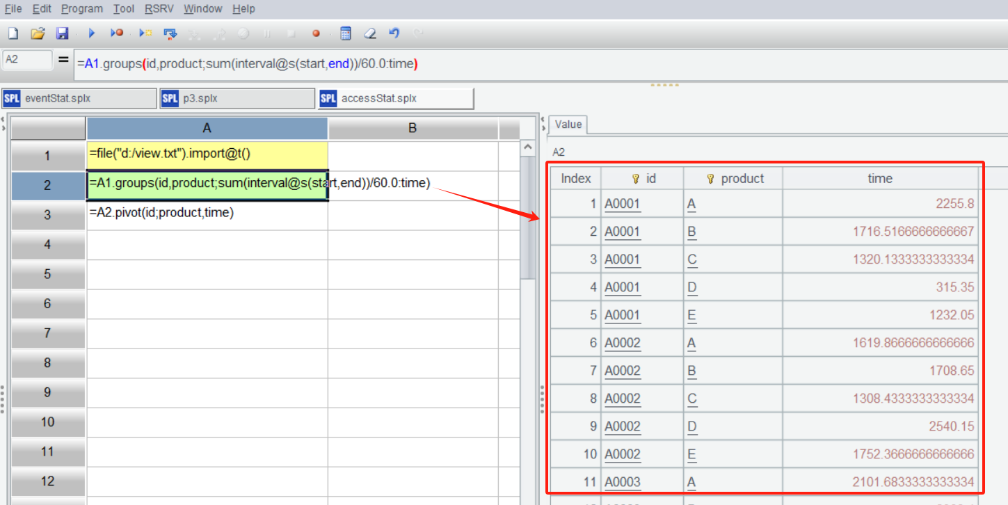
=A1.groups(id,product;sum(interval@s(start,end))/60.0:time) |
3 |
=A2.pivot(id;product,time) |
SPL IDE is highly interactive, allowing for step-by-step execution, and intuitively viewing the result of each step in the right-hand panel at any time. By clicking on cell A2, you can see a summary of the minutes each account spent accessing each product.
A3: Perform a pivot operation on A2. Group by account id, and then pivot each product value into a column name, where the column values are the minutes spent accessing each product.
2. Calculate the daily number of minutes spent accessing products A and B
Because a single access may span multiple dates, you first need to split multiple-data access records into single-day access records, then aggregate the minutes by date and product, and finally perform a pivot operation to get the minutes for products A and B on each date.
Let’s look at the SQL code first:
with recursive days(day) as(
  select min(date(start)) from view
  union all
  select day+interval 1 day from days
    where day<(select max(date(end)) from view)
),
t as (
  select d.day, v.product,
    greatest(v.start, d.day) start,
    least(v.end, d.day+interval 1 day) end
  from days d join view v
    on (v.start>=d.day and v.start<d.day+interval 1 day)
      or (v.end>d.day and v.end<=d.day+interval 1 day)
)
select day,
  sum(if(product='A',timestampdiff(minute,start,end),0)) A,
  sum(if(product='B',timestampdiff(minute,start,end),0)) B
from t
where product='A' or product='B'
group by day;
SQL lacks a function to directly generate a date sequence, requiring the use of a recursive subquery. Moreover, SQL cannot intuitively split each access record by day, you have to associate the view table with the date sequence. These two operations are relatively difficult to understand. Finally, you still need to enumerate grouping values and redefine aggregation calculations to obtain the desired result.
SPL sets are ordered, allowing you to reference data across rows by position when performing calculation on each row. This facilitates a more intuitive approach to splitting out single-day access records and pivoting the data to the expected format.
A |
|
1 |
=file("view.txt").import@t().select(product=="A" || product=="B") |
2 |
=A1.news(periods(start,end).to(2,);product,if(#==1,start,~[-1]):start, ~:end) |
3 |
=A2.groups(date(start):day,product;sum(interval@s(start,end))/60.0:time) |
4 |
=A3.pivot(day;product,time) |
A2: The news function performs calculation on each access record, and the periods function returns the date sequence for the access (including the start and end timestamps). For example, when the start is 2020-01-02 22:41:49 and the end is 2020-01-04 09:32:22, the result of periods(start,end) is:
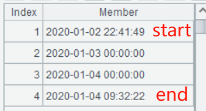
Each of the three time intervals formed by the four time points is contained within a single day.
Use to(2,) to select the end time of each time interval. Then, use these end times as a basis for generating the daily access records.
The parameters after the semicolon in the news function define a new access record. Here, # represents the current index (which time point), ~ represents the current time point, and ~[-1] represents the previous time point. A2 ultimately splits out all access records within a single day (as you can see, the cross-day access records in the red box have been split):
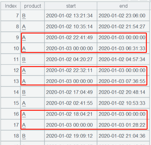
A3: Group by date and product, then aggregate the minutes of each group, and finally pivot the product column in A4.
3. Unify the IDs of users (with the same phone number or email address)
Accounts with the same phone number or email address are deemed to be from the same individual. Now, we want to unify the ids of the same individual to their first registered id (the smallest id).
Prior to unifying the ids, create a new column orid_id to back up the original ids.
Loop through each registered user and compare it with subsequent users. When a match on either phone number or email address is found, unify their ids to the smaller id:
Comparing the original A0001 with subsequent accounts, it is found that A0005 and A0007 are the same individual. Therefore, their ids are unified to A0001;
Comparing the original A0002 with subsequent accounts, it is found that A0003 is the same individual. Therefore, their ids are unified to A0002;
Comparing the original A0003 (now A0002) with subsequent accounts, it is found that A0004 is the same individual. Therefore, their ids are unified to A0002;
Comparing the original A0004 (now A0002) with subsequent accounts, it is found that A0005 (now A0001) is the same individual. Therefore, their ids are unified to A0001;
Comparing the original A0006 with subsequent accounts, it is found that A0008 is the same individual. Therefore, their ids are unified to A0006;
Comparing the original A0008 (now A0006) with subsequent accounts, it is found that A0009 is the same individual. Therefore, their ids are unified to A0006;
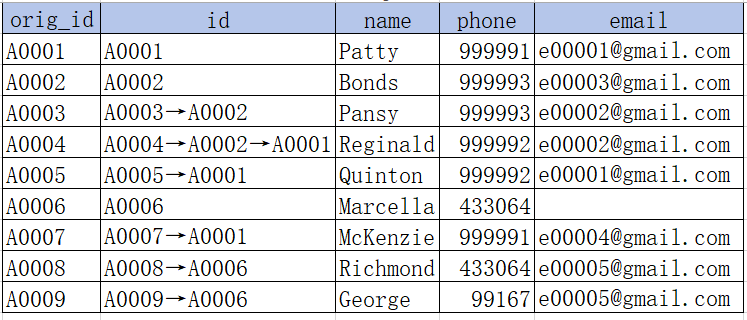
After one traversal, some indirectly related accounts (like A0006 and A0009) have been unified, but others (like original A0002 and A0003, not yet unified with A0001) are left. Therefore, such loop processing needs to be repeated multiple times until no more matching users are found. During the second traversal, original A0003 is unified to A0001.

During the third traversal, A0002 is unified to A0001.

During the fourth traversal, since no matching users are found, the unification process is completed.
Because this approach relies on the order of set members, requires accessing members by position, and necessitates brute-force looping, it cannot be directly implemented in SQL. Furthermore, finding a SQL workaround is difficult, so we won’t attempt to code here.
SPL sets are ordered, allow retrieval of (multiple) members by position, and it is easy to write brute-force looping code following the above processing logic.
A |
|
1 |
=file("user.txt").import@t() |
2 |
=T=A1.derive(id:orig_id) |
3 |
for T.count( |
A2: Add a new column orid_id to back up the ids, then assign the entire table sequence to the variable T.
A3: The outer count function records how many accounts underwent unification in a given loop. As long as the count is greater than 0 (meaning unification occurred), the loop processing will continue.
The inner operation target T[1:] is the set of all accounts after the current account. The count operation on it records how many subsequent accounts have been unified with the current account.
Within the if function, compare the current account (T) with each subsequent account ~ (which can be omitted, for example, phone represents ~.phone). If the comparison indicates the same user, set both account ids (T.id and ~.id) to the smaller id.
A3: There are three nested loops. The outermost for loop is an infinite loop, and the loop’s result is used to determine whether to break the loop.
The T.count loops through all accounts, processing them one by one.
The T[1:].count loops through all accounts after the current account, comparing them with the current account. During calculations, data from all levels can be referenced.
4. Unify IDs and calculate the number of minutes each individual user spent accessing each product
Unify the ids in the user and then associate it with the view based on the original account ids. This enables calculating the number of minutes individual users spend on each product.
The two calculation steps are clear and straightforward. Combining the SPL code from problem 1 and problem 3, with the addition of a join operation in between, will achieve the desired result.
A |
|
1 |
=file("user.txt").import@t() |
2 |
=T=A1.derive(id:orig_id) |
3 |
for T.count( |
4 |
=file("view.txt").import@t() |
5 |
=A4.switch(id,A2:orig_id) |
6 |
=A5.groups(id.id,product;sum(interval@s(start,end))/60.0:time) |
7 |
=A6.pivot(id;product,time) |
A5: Use the switch function to associate the two tables, replace the ids in the view with the corresponding records in the user, forming a two-level table sequence.
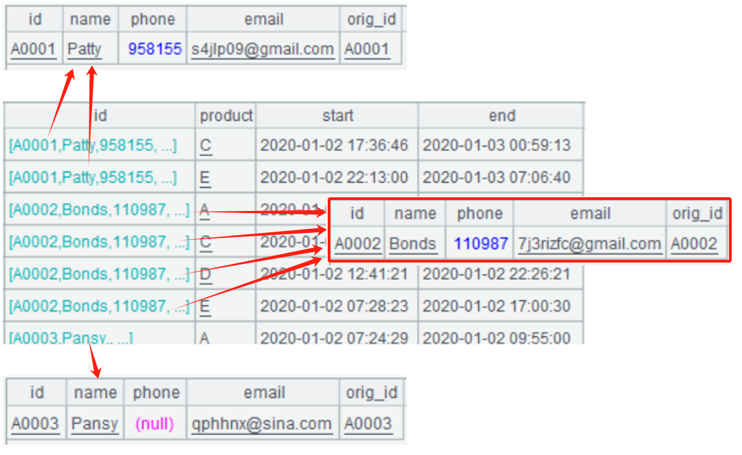
A6: Aggregate the two-level table sequence of A5. The id.id represents the unified ids (similarly, id.name is the account name, and id.orig_id is the original account id).
5. Remove overlapping time spans from the previous aggregation result
After sorting each group of access records by start time, to check for overlaps, first calculate the latest end time x of all previous records. If the current access’s start time is later than x, then there is no overlap. If x falls between the start and end time of the current access, then the time from x to the current access’s end time is not overlapping. If x is later than the current access’s end time, then the entire current access record’s time is overlapping. When performing aggregation, loop through each access record and only accumulate the non-overlapping time spans to the sum.
SPL can perform separate grouping operations to obtain grouped subsets, and then define more complex operations on these grouped subsets. SPL sets are ordered, enabling access to data by position, which facilitates the removal of overlapping time spans following the natural approach described above. This can be accomplished by modifying the previous problem’s cell A6:
A |
|
1 |
=file("user.txt").import@t() |
2 |
=T=A1.derive(id:orig_id) |
3 |
for T.count( |
4 |
=file("view.txt").import@t() |
5 |
=A4.switch(id,A2:orig_id) |
6 |
=A5.group(id.id,product; |
7 |
=A6.pivot(id;product,time) |
A6: Switch to using the independent grouping function group to group by user and product to obtain grouped access record subset ~. Then, sort the records in each subset by start time. Finally, utilize the sum function to calculate the accumulated non-overlapping access time.
The end[:-1] represents the end times of all access records preceding the current access record; max() means finding the latest one from them.
Having calculated x, employ the if() function to determine the three different overlap situations and return the non-overlapping time.
Unlike SQL’s unordered sets, SPL, based on ordered sets, defines many functions with powerful computation capabilities. This makes it easy to code that closely aligns with natural problem-solving approaches, eliminating the need to come up with roundabout, and mentally exhausting alternative workarounds that are often necessary in SQL.
SPL Official Website 👉 https://www.scudata.com
SPL Feedback and Help 👉 https://www.reddit.com/r/esProcSPL
SPL Learning Material 👉 https://c.scudata.com
SPL Source Code and Package 👉 https://github.com/SPLWare/esProc
Discord 👉 https://discord.gg/2bkGwqTj
Youtube 👉 https://www.youtube.com/@esProc_SPL


Chinese Version