

Open-source SPL speeds up intersection calculation of customer groups in bank user profile by 200+ times
Abstract
Bank X divides its over 100 million customers into thousands of groups, hoping to calculate the intersection of any number of customer groups, filter by dimensions, and also hoping to obtain the results in seconds. Click to learn: Open-source SPL speeds up intersection calculation of customer groups in bank user profile by 200+ times
Problem description
In the user profile application of bank X, it is required to calculate the intersection of customer groups. There are thousands of customer groups, and the number of customers in each group is different, varying from hundreds of thousands to over 100 million. In this case, it is required to calculate the common customers of any number (generally 2-10) of customer groups. For example, the customer group for Didi Chuxing has several million customers, and that for mobile banking has tens of millions of customers, it is required to calculate the number of common customers of the two groups.
In addition, for the intersection calculation results, it is also required to filter by dimensions. For instance, for the common customers of Didi Chuxing and mobile banking, it is required to filter by dimensions like gender, age range and region to calculate the final number of customers meeting each dimension condition.
In order to analyze by the time dimension, it has to calculate the results of one year each time. Therefore, the historical data of twelve months need to be saved, one set per month. Calculating the intersection of customers based on detail data of 12 months is called a single task.
Having implemented the intersection calculation of customer groups based on a well-known OLAP Server product on Hadoop, Bank X found the performance is very poor. In this calculation, a virtual machine cluster with 100 CPUs (cores) was used, and it took around 2 minutes to complete a single task on average. However, the expected performance goal is to complete 10-20 single tasks concurrently in 10 seconds, and hence the gap is extremely large.
Using the pre-calculating method recommended by the OLAP Server can meet the performance requirements, which works in a way that pre-calculate the intersection of customer groups, save the calculation results, and filter by the dimensions based on the results. However, for thousands of customer groups, there will be over 10 million of combinations when just calculating the intersection of any two customer groups. Although it can barely be stored, it is an impossible task to save in advance when calculating the intersection of more customer groups.
Solution
Step 1, in-depth understanding of the characteristics of data and calculations, and analysis of performance bottlenecks.
Each dimension value of customer is unique, and each customer can be stored in one record, 100 million customers are 100 million records.
There is no hierarchical relationship between dimensions, and the number of attributes of a dimension is generally several to dozens. For example, the number of attributes of gender dimension is two, and that of age range dimension is about a dozen. The total number of dimensions involved in filtering is ten to twenty.
A customer belongs to 10 customer groups on average. If the database table is used to store, the customer-customer group table will have over one billion records, see the following figure for the table structure.
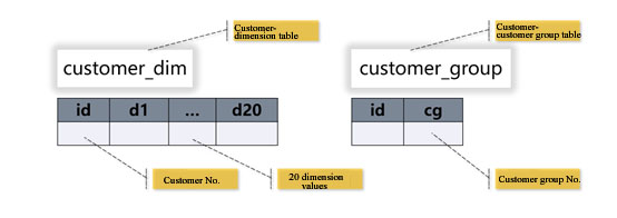
The SQL statement for calculating the intersection of customer groups and filtering by dimensions is simplified as:
select count(*) from (
select count(g.cg) from customer_group g
left join customer_dim d on g.id=d.id
where g.cg in ('18','25')
and d.d2 in ('2','4')
and d.d4 in ('8','10','11')
group by g.id
having count(g.cg)=2
)
In this SQL statement, there is a JOIN that may tie down the computing performance, but if two large tables are JOINed into a wide table, more than ten times redundancy may occur to the same dimension value, in that case, the query speed will be further decreased. If using the comma-separated string to store multiple customer group numbers into a field cg, although the dimension value redundancy can be avoided, it needs to perform the string splitting calculation, and the speed will still be very slow in the case of large data amount. For example, “18, 25, 157” in field cg means that the customer belongs to three customer groups, it needs to use the substrings to compare when calculating the intersection, and hence the amount of calculation is still very large. It is found, after some experiments, that in the current technical environment, continuing to use this table structure and such SQL statement can still obtain the best performance. Although this JOIN involves large tables, it has filter conditions, after filtering, it will become small table in-memory JOIN, and the performance loss is not very serious. The more important operation bottleneck is the IN condition in filter conditions, which is a computationally inefficient set operation and is related to the number of IN’s enumeration values, the more enumeration values, the worse the performance.
Step 2, determine the optimization scheme.
Complete data needs to be saved every month, but the memory capacity of bank X's standard virtual machine is only 16G, it cannot hold the data of even one month, and hence the all-in-memory calculation cannot be implemented. In this case, we need to read data from external storage and calculate. To do so, we should first consider reducing the amount of data storage and access. If two tables are still used, it needs to be read them separately and does association, which will increase the amount of access and calculation. Therefore, we consider merging the two tables into one, with one row of data per customer, and storing the dimension attributes and the customer groups at the same time. In this way, the total amount of data is equal to the number of customers. In particular, the dimension attributes should be stored in integers, as the amount of storage and calculation is smaller than that of strings.
There are thousands of customer groups, if they are saved as integers, the amount of data will be huge. However, the attribute of customer group belongs to tag attribute with only two states, yes and no, which can be saved with just one bit. A small-integer-type binary number represents 16 bits, and each bit can represent one customer group. For the convenience of calculation, we use 15 bits of a small integer to save customer group tags, and thus 600 small integers can save 9000 customer group tags.
In the data table, we use 600 fields c1 to c600, each of which represents the location of 15 customer groups. 0 represents that it doesn’t belong to this customer group, while 1 represents that it belongs to this customer group. When calculating the intersection of two customer groups, take at most 2 columns; similarly, when calculating the intersection of n customer groups, take at most n columns. Since the columnar storage is adopted, when n is less than 10, the amount of reading can be greatly reduced.
The dimension fields d1 to d20 no longer store the corresponding dimension values, but the sequence numbers of dimension value in dimension list. For example, d2 is the age dimension, the age range of customer 001 is 20-30, and the corresponding enumeration value sequence number in the age dimension list is 3, then set the d1 field of this customer to 3.
When filtering by dimensions, calculate the entered age range condition as a boolean sequence, and the length of sequence is the number of attributes of age range dimension. If the age range condition is 20-30, set the third member in the sequence to true and the others to false.
While performing the condition filtering to the newly stored file, when traversing the row of customer 001, if the value taken in d1 is 3, and the third element of boolean sequence is true, then customer 001 meets the filtering conditions.
This algorithm is called the dimension of boolean sequence, and the dimension value of each customer can be saved with only 20 integers in one row of data. The advantage of this algorithm is that there is no need to judge IN when querying. As mentioned above, the performance of IN is poor and related to the number of enumeration values, while the judgment of dimension of boolean sequence is a constant time.
According to the new idea, this algorithm is mainly to perform the bitwise calculation to the large columnar storage data table, and do the filter traversing to the dimension of boolean sequence. There are many filter conditions of AND relationships, involving multiple fields. When traversing, we can first read and compute the fields corresponding to the first few conditions. If they meet these conditions, read the fields corresponding to subsequent conditions; if not, the subsequent fields are no longer read. Such algorithm, called pre-cursor filtering, can effectively reduce the amount of data read.
Step 3, select the technical route.
Only very few commercial databases’ SQL can support bit operation, but it does not match the whole technical system; if such databases was used, it would result in a very cumbersome architecture. Adding UDF to the SQL of the current platform to implement bit operation would make the complexity of code very high. If the optimization was performed based on the current SQL system, it would be extremely costly.
If the high-level language such as Java or C++ was used, the above algorithms could certainly be implemented; however, just like adding UDF, the code would still be very complex, and it would need hundreds or even a thousand of lines of code to implement such algorithms. Too large amount of coding will lead to too long project period, hidden trouble with code errors, and it is also difficult to debug and maintain.
For example, objectification is needed when Java reads data from the hard disk; however, Java is slow to generate objects. If the above-mentioned pre-cursor filtering is not used, many columns need to be read into memory before judging, resulting in the generation of a lot of useless objects, this will have a great impact on the performance. If coding in Java to implement pre-cursor filtering algorithm from the very beginning, it takes both time and effort.
The open-source esProc SPL provides support for all the above algorithms, including mechanisms such as the high-performance compression columnar storage, boolean, bitwise calculation, small integer objects and pre-cursor filtering, which allows us to quickly implement this personalized calculation with less amount of code.
Step 4, execute the optimization scheme. Coding in esProc SPL to combine the dimension attributes of customers in the data with the customer groups they belong to, and store them in esProc high-performance binary columnar storage files according to the new storage structure. At the beginning of each subsequent month, extract the newly added data, and store them in the same way.
Then write the SPL code for query, convert the input conditions (dimension attributes, and customer groups for calculating intersection) to the format required by boolean dimension and bitwise calculation, and perform the pre-cursor filtering and counting to the new storage structure.
esProc provides JDBC driver for external application, just like calling the stored procedure of database, the driver allows the front-end applications to call esProc, we can input the parameters and obtain the query results.
Actual effect
After about two weeks of coding and testing, the actual optimization effect is very obvious. It only takes 4 seconds to execute a query on 12 months of data with a 12-CPU (cores) virtual machine; while the original 100-CPU (cores) virtual machine needs 120 seconds to execute the same query, thus improving the performance by 250 times (100 CPUs*120 seconds ÷ 12 CPUs*4 seconds). To further achieve the desired performance goal, that is, perform 10-20 single tasks concurrently within 10 seconds, the required resource can be completely controlled within 100-CPU (cores).
This scheme does not need to pre-calculate, and can query on the detail data directly, and thus it is very flexible. To calculate the intersection of any number of customer groups, the speed will be the same, thereby completely solving the performance problem of the intersection operation of customer groups.
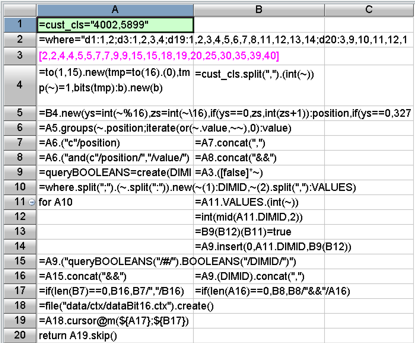
In terms of development difficulty, SPL has made a lot of encapsulations, provided rich functions, and built-in the basic algorithms required by the above scheme. The SPL code corresponding to the algorithms mentioned above has only 20 lines:
Postscript
To solve the performance optimization problem, the most important thing is to design a high-performance computing scheme to effectively reduce the computational complexity, thereby ultimately increasing the speed. Therefore, on the one hand, we should fully understand the characteristics of calculation and data, and on the other hand, we should have an intimate knowledge of common high-performance algorithms, only in this way can we design a reasonable optimization scheme according to local conditions. The basic high-performance algorithms used herein can be found at the course: , where you can find what you are interested in.
Unfortunately, the current mainstream big data systems in the industry are still based on relational databases. Whether it is the traditional MPP or HADOOP system, or some new technologies, they are all trying to make the programming interface closer to SQL. Being compatible with SQL does make it easier for users to get started. However, SQL, subject to theoretical limitations, cannot implement most high-performance algorithms, and can only face helplessly without any way to improve as hardware resources are wasted. Therefore, SQL should not be the future of big data computing.
After the optimization scheme is obtained, we also need to use a good programming language to efficiently implement the algorithms. Although the common high-level programming languages can implement most optimization algorithms, the code is too long and the development efficiency is too low, which will seriously affect the maintainability of the program. In this case, the open-source SPL is a good choice, because it has enough basic algorithms, and its code is very concise, in addition, SPL also provides a friendly visual debugging mechanism, which can effectively improve development efficiency and reduce maintenance cost.
SPL Official Website 👉 http://www.scudata.com
SPL Feedback and Help 👉 https://www.reddit.com/r/esProc
SPL Learning Material 👉 http://c.scudata.com
SPL Source Code and Package 👉 https://github.com/SPLWare/esProc
Discord 👉 https://discord.gg/ydhVnFH9
Youtube 👉 https://www.youtube.com/@esProc_SPL


Chinese version