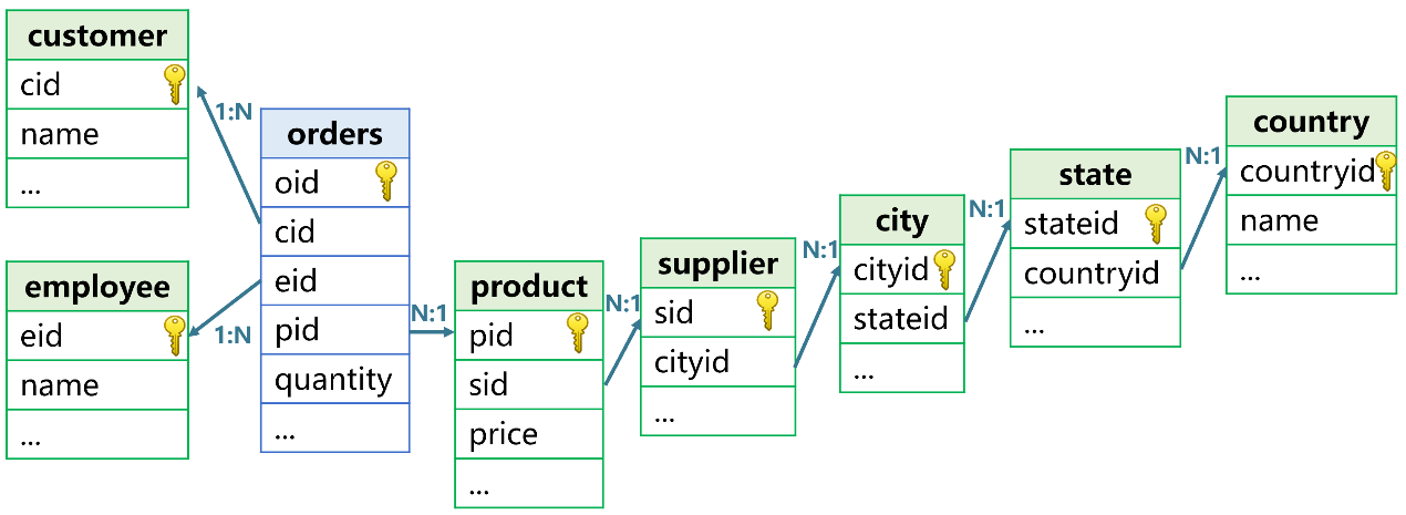
In a multidimensional application, a fact table always has a lot of dimension tables. As the following shows, the orders table has a series of dimension tables:

 

The association between any of the dimension tables and the fact table is the JOIN defined in SQL. Technically, databases use the HASH JOIN algorithm to achieve the joins, implementing one at a time. N times of HASH JOIN are needed when there are N joins, and each intermediate result set will be retained for use in the next join. The computing process is complex and involves multiple traversals, markedly dragging down the performance.

When there are a lot of dimension tables in different levels, the database optimizer often cannot get the best order for implementing the joins. Different orders produce different intermediate result sets and numbers of copy operations. If each join involves the big table, there will be huge amounts of extra computations, leading to a sharp decrease in performance. Besides, it is hard to implement HASH JOIN algorithm with the parallel processing in this context and thus the latter’s advantages cannot be fully used to increase performance.

 

Usually, the size of all dimension tables is relatively small and can fit into the memory. If we can load them into the memory at the startup of the multidimensional analysis system, create indexes on them, and establish data association between them in advance, we then just need to join the fact table and the joined dimension tables. This will shave off one round of hash value computation from the whole process and get rid of the join implementation order issue, as well as making a clear-cut distinction between the fact table and the dimension tables – making it easy to implement parallel processing by first segmenting the fact table.

The open-source esProc SPL is suitable for achieving the above algorithm. It has the following code:

l. Initialize the system:

A1=file("customer.btx").import@b().keys@i(cid)

      // Import dimension table customer and create index on it

A2=file("product.btx").import@b().keys@i(pid).switch(sid,file("supplier.btx").import@b().keys(sid))      

      // Pre-join dimension tables product and supplier

>env(customer,A1),env(product,A2)

2. Perform multidimensional analysis:

A1=file("orders.ctx").open().cursor@m(pid,cid,quantity).switch(pid,product;cid,customer)

      // Search for the matching records from desired dimension tables and join the fact table with them, and perform analysis with parallel processing

A2=A1.select(pid.sid.name=="raqsoft.com").groups(cid.city;sum(pid.price*quantity))

      // Slice the pre-joined fact table and dimension tables by supplier id, and group and summarize records according to cities customers come from

 

If the fact table is small enough to be wholly loaded into the memory at the startup of the multidimensional analysis system and the joins between it and the desired dimension tables can be created in advance, we can reference fields of dimension tables directly at computation without any HASH JOIN computation, improving performance more notably.

l．Initialize the system:

A1=file("customer.btx").import@b().keys@i(cid)

      // Set the primary key, with index attached, on dimension table customer

A2=file("product.btx").import@b().keys@i(pid).switch(sid,file("supplier.btx").import@b().keys(sid))

      // Pre-join dimension tables product and supplier

A3=file("orders.btx").import@b().switch(cid,A1;pid,A2)

      // Multilevel pre-join between the fact table orders and dimension table customer and dimension table product

>env(orders,A3)      // Store the result table of pre-joining the fact table and dimension tables in a global variable for later use

2. Perform multidimensional analysis:

orders.select(pid.sid.name=="raqsoft.com").groups(cid.city;sum(pid.price*quantity))

      // Slice the pre-joined fact table and dimension tables by supplier id, and group and summarize records according to cities customers come from

 

If the fact table is huge, we can first numberize it by converting all dimension fields to the ordinal numbers of records in the corresponding in-memory dimension tables. Then we load the fact table to the memory in batches and use the dimension field values – now ordinal numbers of the corresponding dimension table – to get matching records of the dimension table directly. The performance is much higher than that of using the index-based searching, and almost as good as that brought about by the in-memory pre-join.

l. Numberize the fact table:

A1=file("orders-original.ctx")                    // Open the original data table

A2=A1.reset@n(file("orders.ctx"))              // Create a new table by copying the original table’s structure

A3=A1.open().cursor().run(pid=file("product.btx").import@b().keys@i(pid).pfind(pid),cid= file("customer.btx").import@b().keys@i(pid).pfind(cid))

> file("orders.ctx").append(A3)                  // Convert dimension field to ordinal numbers of records in the corresponding dimension table and store data to the new table

2. Initialize the system:

A1=file("product.btx").import@b().switch(sid,file("supplier.btx").import@b().keys(sid))

      // Pre-join dimension tables product and supplier

>env(customer,file("customer.btx").import@b()),env(product,A1)

      // Store the result table of pre-join in a global variable without creating indexes on dimension tables customer and product, so that memory usage can be reduced

3. Perform multidimensional analysis:

A1=file("orders.ctx").open().cursor(pid,cid,quantity).switch(pid,product:#;cid,customer:#)

      // Use the ordinal numbers to locate dimension table records

A2=A1.select(pid.sid.name=="raqsoft.com").groups(cid.city;sum(pid.price*quantity))

      // Same code for multidimensional analysis as that using the in-memory pre-join

 

Relational databases cannot achieve the above algorithms because they do not have the concept of object pointer and Cartesian-product-based SQL JOIN does not postulate the uniqueness of records referenced by the foreign key. Engineering optimization is the best they can do in an effort to achieve similar algorithms, and to some extent, improves their abilities to implement multi-dimension-table joins at one time and parallel processing. The optimization produces good results only for two-table joins. When a join involves more tables and multiple types of joins, this kind of database optimization begins to lose its strength. That’s why when the number of dimension tables increases to four or five database, performance of multidimensional analysis starts to plummet. In fact, according to the previous explanations, even SQL-based in-memory databases struggle with multidimensional analysis involving a lot of dimension tables. The only effective way to obtain high performance for multidimensional analysis is to look at join operations differently and employ new computational strategies.