

How to merge Excel Sheets horizontally
Horizontal merging is also a common Excel problem encountered in work, and it is also quite troublesome to do in Excel, and many people do not know how to do it. For example, how to do one-on-one, how to do one-to-many, how to do with different number of rows, and how to do with multiple merge conditions. This article provides detailed solutions for these scenarios. And the method here is definitely the most efficient one that you have found.
Let’s skip the formalities and get straight to business.
Firstly, we need to use a tool called esProc SPL, which is a software specifically designed to handle structured table data. It has powerful computing capabilities and is easy to use. After downloading, double-click to install. The examples in this article are all provided with source code and can be copied and pasted for use.
Download address: esProc Desktop Download
1. One on one merge
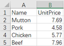
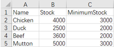
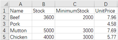
As shown in the figure, there are two tables, namely the price table and inventory table for certain meat products. Now, we need to merge the two tables horizontally.
Before merging:
Meats.xlsx
MeatStock.xlsx
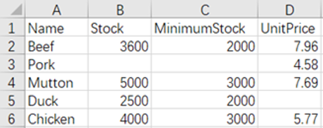
(1)Horizontal merge, retain all rows (full join)
Merge according to Name, retain all rows after merging
After merging:
Implementation code:
| A | |
|---|---|
| 1 | =file(“Meats.xlsx”).xlsimport@t() |
| 2 | =file(“MeatStock.xlsx”).xlsimport@t() |
| 3 | =join@f(A1:Price,Name;A2:Stock,Name) |
| 4 | =A3.new([Price.Name,Stock.Name].ifn():Name,Stock.Stock,Stock.MinimumStock,Price.UnitPrice) |
| 5 | =file(“MeatsPriceStock.xlsx”).xlsexport@t(A4) |
A3 join@f() represents full join, retaining all rows
A4 The bold code means selecting non null Name values
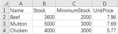
(2)Horizontal merge, only retaining duplicate rows (inner join)
Merge according to Name, only retaining rows common to both files
After merging:
Implementation code:
| A | |
|---|---|
| 1 | =file(“Meats.xlsx”).xlsimport@t() |
| 2 | =file(“MeatStock.xlsx”).xlsimport@t() |
| 3 | =join(A1:Price,Name;A2:Stock,Name) |
| 4 | =A3.new(Stock.Name,Stock.Stock,Stock.MinimumStock,Price.UnitPrice) |
| 5 | =file(“MeatsPriceStock.xlsx”).xlsexport@t(A4) |
A3 inner join, retaining common rows
(3)Only retain the rows of the first file (left join)
Merge according to Name, retain the rows of the first file after merging
After merging:
Implementation code:
| A | |
|---|---|
| 1 | =file(“Meats.xlsx”).xlsimport@t() |
| 2 | =file(“MeatStock.xlsx”).xlsimport@t() |
| 3 | =join@1(A1:Price,Name;A2:Stock,Name) |
| 4 | =A3.new(Price.Name,Stock.Stock,Stock.MinimumStock,Price.UnitPrice) |
| 5 | =file(“MeatsPriceStock.xlsx”).xlsexport@t(A4) |
A3 @1 is a left join, please note that here is the number 1, not the letter l
(4)Multiple merge conditions, only retaining the rows of the first file (left join)
As shown in the following figure, according to the conditions of Region and Name, retaining the rows of the first file, and merge the two tables horizontally.
Before merging:
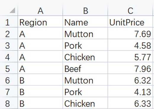
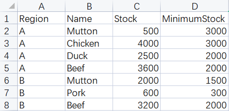
After merging:
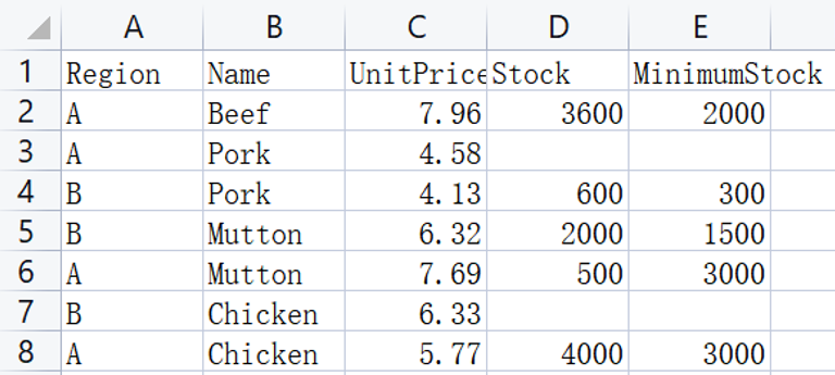
Implementation code:
| A | |
|---|---|
| 1 | =file(“Meats.xlsx”).xlsimport@t() |
| 2 | =file(“MeatStock.xlsx”).xlsimport@t() |
| 3 | =join@1(A1:Price,Region,Name;A2:Stock,Region,Name) |
| 4 | =A3.new(Price.Region,Price.Name,Stock.Stock,Stock.MinimumStock,Price.UnitPrice) |
| 5 | =file(“MeatsPriceStock.xlsx”).xlsexport@t(A4) |
A3 can implement multi condition merging by adding condition field names to the join() function
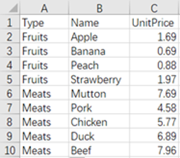
2. One to many merge
Before merging:
Types.xlsx
Foods.xlsx
After merging:
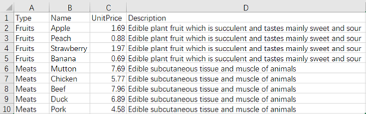
It can be implemented using full join.
Implementation code:
| A | |
|---|---|
| 1 | =T(“Types.xlsx”) |
| 2 | =T(“Foods.xlsx”) |
| 3 | =join@f(A1:Type,Type;A2:Food,Type) |
| 4 | =A3.new(Food.Type,Food.Name,Food.UnitPrice,Type.Description) |
| 5 | =T(“FoodsDescription.xlsx”,A4) |
A3 @f is a full join.
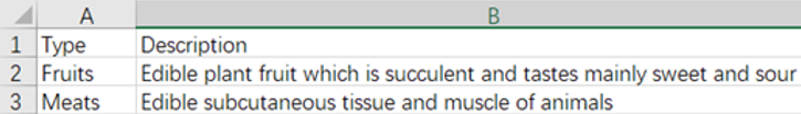
If the description of the major categories Fruits and Meats is expected to only appear once, as shown in the figure
After merging:
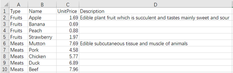
You can use the align() function.
Implementation code:
| A | |
|---|---|
| 1 | =T(“Types.xlsx”) |
| 2 | =T(“Foods.xlsx”) |
| 3 | =A1.align(A2:Type,Type) |
| 4 | =A2.new(Type,Name,UnitPrice,A3(#).Description) |
| 5 | =T(“FoodsDescription.xlsx”,A4) |
A3 align indicates that A1 is aligned to A2, with the alignment criteria being the Type column of A2 and the Type column of A1. If A2 has duplicate data, only the first row is aligned.
Using SPL, complex Excel operations can be done with just a few lines of code.
In addition, the syntax of SPL functions is simple, in line with natural logical thinking, and it is not difficult to understand.
Of course, the functions of SPL are not limited to this, and it is not a problem to SPL for Excel operations in various complex scenarios.
For those in need, you can refer to Desktop and Excel Data Processing Cases . Ninety per cent of Excel problems in the workplace can find answers in this book. The code in the book can basically be copied and used with slight modifications.
SPL Official Website 👉 https://www.scudata.com
SPL Feedback and Help 👉 https://www.reddit.com/r/esProc_Desktop/
SPL Learning Material 👉 https://c.scudata.com
Discord 👉 https://discord.gg/2bkGwqTj
Youtube 👉 https://www.youtube.com/@esProcDesktop
Linkedin Group 👉 https://www.linkedin.com/groups/14419406/


Chinese version