Problem description

Data structure and data scale

Customer - dimension table (cust_dim):

Field name	Field type	Field meaning	Sample data
id	Number	Customer number	18765
d1	Number	Dimension 1	12
…	…	…	…
d10	Number	Dimension 10	3
…	…	…	…

This table contains a total of 100 million customers, each of which has a unique id.

Each customer has 10 dimensions. For example, d2 is the age group dimension, which corresponds to 8 enumeration values, indicating the value range of d2 is 1 to 8.

d4 is the educational background dimension, which corresponds to 12 enumeration values, indicating the value range of d4 is 1 to 12.

Customer - customer group table (cust_group):

Field name	Field type	Field meaning	Sample data
id	Number	Customer number	18765
cg	Number	Customer group number	304
…

A customer belongs to multiple customer groups (approximately 10 on average) and there are 1,000 customer groups in total. This table contains about 1 billion records.

Each of the two tables will generate a full data snapshot every month. Since the actual calculations are based on one month’s data rather than the data spanning months, we take one month’s data as an example to practice.

Condition and expectation

The calculation of customer profile involves the intersection of customer groups and filtration by dimensions.

1. Intersection of customer groups refers to finding the customer who belongs to two or three groups at the same time (like the customer who belongs to both groups 18 and 25).

2. Filtration by dimensions refers to finding the customer whose dimension values are within a specified range (such as the customer whose d2 value is 2 or 4 and whose d4 value is 8, 10, or 11).

3. The final result should be the number of deduplicated customers that satisfy both 1 and 2 above.

Coding in SQL is roughly as follows:

select count(*) from (
select count(g.cg) from customer_group g
                              left join customer_dim d on g.id=d.id
             where g.cg in ('18','25')
             and d.d2 in ('2','4')
             and d.d4 in ('3','6','10')
             group by g.id
             having count(g.cg)=2
)

It is desired that 10-20 such calculations can be completed concurrently within 10 seconds using as few hardware resources as possible.

When using a certain well-known commercial data warehouse on HADOOP and utilizing a virtual machine cluster consisting of 100 CPUs (cores) to calculate the intersection of two customer groups, it took around 2 minutes on average, yet it failed to obtain result when calculating the intersection of three or more customer groups.

Also, using the pre-calculation method recommended by this commercial data warehouse does not work because the result of calculating the intersections of any two customer groups among 1000 groups, plus any combination of 10 dimensions is already very large, and it is impossible to save the intersections of three or more customer groups in advance.

Problem analysis

IN calculation

Filtration by dimensions is actually the IN operation for a set. The performance of IN operation is poor, mainly owing to the fact that it involves many comparison calculations. Specifically, to determine whether the field d is contained in a value set, it needs to compare d with the members of value set by 1 to n times if the sequential search is adopted. Even when the given set of values is ordered and the binary search can be used, it still needs to compare by many times. When the amount of data is huge, the number of comparisons will be very large, resulting in very slow in judging IN condition and, the larger the value set, the slower the speed.

The boolean dimension sequence of SPL can eliminate the comparison calculation of IN. First determine the list of possible values of the IN field (the field before writing as IN condition). Generally, the number of possible values is not too large, so the list will not be too long. Then convert the original data, replacing the values of the IN field with the sequence numbers (positions) of the corresponding record in the list, and storing these sequence numbers as a new data.

When judging whether the new data meets the IN condition, a set of boolean values with the same length as the list needs to be generated first, and the ith value in the set is determined by judging whether the ith member in the list is contained in the value set of IN field, it is true if the ith member is contained, otherwise it is false. When traversing the data, use the value of the IN field (the sequence number in the list) to take the member of boolean value set. If it is true, it indicates the filter condition is satisfied, otherwise the filter condition is not satisfied.

The boolean dimension sequence is to convert “comparison of set values” to “reference of sequence number” in essence, which eliminates the comparison calculation and greatly improves performance. Moreover, the computation time is independent of the size of value set and won’t increase as the number of enumeration values in IN condition grows.

In contrast, RDB does not support directly accessing the members of a set by sequence number (position) in general, and instead, it needs to use a transitional approach, i.e., access the members of set by associating tables, which will cause more complex JOIN operation, and hence the said optimization method cannot be directly implemented.

Association of large tables

The association of the two large tables ‘cust_dim’ and ‘cust_group’ is one of the main reasons that slow down the overall performance. If the two tables are joined as a wide table, more than ten times redundancy may occur to the same dimension value, and the query speed will be further decreased.

If the number of customer groups is not too large, we can consider storing each group as a field, and using 0 and 1 to represent whether a customer belongs to a group. However, now there are 1000 customer groups, exceeding the maximum field number of database table (usually 256 or 512).

The columnar file of SPL can accommodate much more columns, up to a thousand of columns.

Moreover, we can also utilize the bitwise storage mechanism to be described below and use a binary bit to represent customer group. In this way, two large tables can be merged, which not only eliminates the association of two large tables but avoids too many columns.

Binary tag

Using 0 and 1 to represent whether a customer belongs to a certain customer group is actually the binary tag. SPL supports bitwise storage of binary tag, which means to use a single binary bit to store a tag. Combining multiple tags into a 16- or 32- or 64-bit integer can significantly reduce the number of columns in the table and the storage amount (reducing by 16-64 times compared to conventional storage methods).

SPL provides a special performance optimization mechanism for 16-bit small integer, so it is recommended to use small integer to implement bitwise storage of binary tag.

Customer groups correspond to many binary tags (one thousand). Bitwise storage of these tags can effectively reduce the amount of data reading and computation. A 16-bit integer can store 16 binary tags that need to calculate conditions, we just need to read and calculate once to get the intersection of 16 customer groups.

Although some databases now support bit-based operations, writing SQL syntax is still relatively cumbersome. SPL provides pseudo table objects that make the operation of combing binary tags transparent. Programmers can continue to operate on individual tag fields, which are actually converted by SPL to certain bits of a 16-bit integer.

Practice process

Prepare data

	A	B
1	=file("cust_dim.txt")
2	=file("cust_group.txt")
3	>movefile@y(A1),movefile@y(A2)
4	for 1000	=to(100000).new((#A4-1)*100000+~:id,rand(20)+1:d1,rand(8)+1:d2,rand(30)+1:d3,rand(12)+1:d4,rand(25)+1:d5,rand(18)+1:d6,rand(50)+1:d7,rand(20)+1:d8,rand(35)+1:d9,rand(40)+1:d10)
5		=A1.export@at(B4)
6		=B4.new(id,to(8+rand(4)).new(rand(1000)+1:cg):cgroup)
7		=B6.news(cgroup;id,cg)
8		=A2.export@at(B7)

This code generates two text files ‘cust_dim’ and ‘cust_group’ to serve as the raw data exported from business system. Each of them contains one month’s data. The data volume of ‘cust_dim’ is 100 million, and that of the ‘cust_group’ is 1 billion.

Data preprocessing

	A	B
1	=file("cust_dim.txt").cursor@t().sortx(id)
2	=file("cust_group.txt").cursor@t().sortx(id,cg)
3	=A2.group(id;~.(cg):cgs,1008.(false):t)
4	=A3.run(cgs.(t(~)=true))
5	=1008.("t("/~/"):cg"/~).concat@c()	=A4.derive(${A5})
6	=B5.joinx@m(id,A1:id,d1,d2,d3,d4,d5,d6,d7,d8,d9,d10)
7	=(1008\16).("bits"/~).concat@c()
8	=file("cust_dim_group.ctx").create@y(#id,d1,d2,d3,d4,d5,d6,d7,d8,d9,d10,${A7})
9	=1008.("cg"/~).group((#-1)\16).("bits@b("/~.concat@c()/"):bits"/#)
10	=A6.new(id,d1,d2,d3,d4,d5,d6,d7,d8,d9,d10,${A9.concat@c()})
11	=A8.append(A10)	>A8.close()

This code preprocesses the text files, implements the merging of two tables, eliminates the association of large tables, and implements the bitwise storage of binary tags.

A1, A2: sort the ‘cust_dim’ by id, and sort the ‘cust_group’ by id and cg. Since the raw data are usually generated and stored in chronological order, and they are not ordered by id in general, a sorting operation is required here;

A3: group the ‘cust_group’ in order by id, merge each cg group into a set field cgs, and generate a new set field t, which contains 1008 false;

Since the number of customer groups is 1000, which is not divisible by 16, we increase the number to 1008 here so that these customer groups can be stored with 63 16-bit integers. The extra number will not affect the calculation.

A4: assign true to the member at corresponding location in t based on the value of the customer group number cg in cgs;

A5: dynamically generate the code that produces new fields; B5: dynamically generate new fields. In fact, the code in B5 is roughly as like: =A4.derive(t(1):cg1,t(2):cg2,t(3):cg3,…,t(1008):cg1008).
The purpose is to define the 1008 boolean values in t as new fields cg1 to cg1008.

A6: merge B5 and A1 in order by id. Since B5 is also ordered by id and unique, the two tables are now in the homo-dimension relationship;

A7: dynamically generate names for 63 fields; A8: define composite table. In fact, the code in A8 is roughly like: =file(“cust_dim_group.ctx”).create@y(#id,d1,d2, …,d10, bits1,bits2,bits3,…,bits63).

A9: dynamically generate conversion code, which aims to convert 1008 boolean fields to 63 hexadecimal integer fields for bitwise storage;

A10: the actual conversion code is roughly as follows:

=A6.new(id,d1,d2,…,d10,
bits@b(cg1,cg2,...,cg16):bits1,
bits@b(cg17,cg18,...,cg32):bits2,
...
bits@b(cg993,cg994,...,cg1008):bits63
)

Assume the customer whose id is 1 belongs to cg18 and cg25, then the second hexadecimal field ‘bits2’ is assigned the binary number: 0100000010000000, where the 2nd and 9th bits from the left correspond to cg18 and cg25 respectively.

Converting this binary number to decimal gives 16512.

A11: insert the converted data into the composite table in A8; B11: close the composite table.

Customer profile calculation

	A	B
1	=arg_cg="18,25"
2	=arg_d2="2,4"	=arg_d4="3,6,10"
3	=arg_cg.split@c().(int(~)).group@n(~\16+1)
4	=A3.(~.sum(shift(1,~%16-16)))
5	=A4.pselect@a(~>0)
6	=A5.("and(bits"/~/","/A4(~)/")=="/A4(~))
7	=d2s=8.(false)	=arg_d2.split@c().(A7(int(~))=true)
8	=d4s=12.(false)	=arg_d4.split@c().(A8(int(~))=true)
9	=file("cust_dim_group.ctx").open().cursor(id;d2s(d2) && d4s(d4) && ${A6.concat("&&")})
10	=A9.skip()

A1, A2, and B2 are the parameters passed in, respectively representing the customer group number set, enumeration value set of d2, and enumeration value set of d4. We can see that the number of members in the customer group number set and the enumeration value set is changeable. For example, to calculate the intersection of three or more customer groups, we just need to add the comma-separated members in the string.

In practice, the parameters are often dynamic and can be passed in as json string and then parsed in SPL code.

A3: group the customer number parameters by multiple of 16. 18 and 25 are assigned to group 2, and subsequent queries will correspond to bits2.

A4: calculate the binary number corresponding to cg through shift and summation. The bitwise storage of 18 and 25 corresponds to integer 16512;

A5: find the location of the member that is greater than zero, and the result here is 2;

A6: dynamically generate the bitwise AND calculation code, which is and(bits2,16512)==16512 in this practice. If the result of the bitwise AND operation between bits2 and 16512 (binary number 0100000010000000) is still 16512, then bits2 meets the condition of containing cg18 and cg25.

A7, A8: generate the boolean dimension sequence for ds2 and ds4;

A9: use bitwise AND and boolean dimension to filter the composite table cursor. The actual code to be executed is:

=file("cust_dim_group.ctx").open().cursor(id;d2s(d2) && d4s(d4)
&& and(bits2,16512)==16512)

A10: since the ids in the composite table are unique and non-repetitive, the number of deduplicated ids can be obtained by counting the cursor directly.

Use pseudo table

We can use the pseudo table object of SPL Enterprise Edition to encapsulate the bitwise storage mechanism and simplify code.

The code to preprocess the data should be changed to:

	A	B
1	=file("cust_dim.txt").cursor@t().sortx(id)
2	=file("cust_group.txt").cursor@t().sortx(id,cg)
3	=A2.group(id;~.(cg):cgs,1008.(false):t)
4	=A3.run(cgs.(t(cgs.~)=true))
5	=1008.("t("/~/"):cg"/~).concat@c()	=A4.derive(${A5})
6	=B5.joinx@m(id,A1:id,d1,d2,d3,d4,d5,d6,d7,d8,d9,d10)
7	=(1008\16).("bits"/~).concat@c()
8	=file("cust_dim_group.ctx").create@y(#id,d1,d2,d3,d4,d5,d6,d7,d8,d9,d10,${A7})
9	=(1008\16).(16.("\“cg"/((get(1)-1)*16+~)/"\”").concat@c())
10	=(1008\16).("{name:\“bits"/~/"\”,bits:["/A9(#)/"]}").concat@c()
11	=[{file:"cust_dim_group.ctx", column:[ {name:"d2",enum:"ages",list:["0-10","11-20","21-30","31-40","41-50","51-60","61-70","71-"]}, {name:"d4",enum:"edu",list:["edu1","edu2","edu3","edu4","edu5","edu6","edu7","edu8","edu9","edu10","edu11","edu12"]}, ${A10} ] }]
12	=p_cust_dim_group=pseudo(A11)
13	=p_cust_dim_group.append(A6)	>p_cust_dim_group.close()

A1 to A8 remain unchanged.

A9 to A11 prepare the json strings that define pseudo table in three steps, which are roughly as follows:

[{file:"cust_dim_group.ctx",
column:[
{name:"d2",enum:"ages",list:["0-10","11-20","21-30","31-40","41-50","51-60","61-70","71-"]},
{name:"d4",enum:"edu",list:["edu1","edu2","edu3","edu4","edu5","edu6","edu7","edu8","edu9","edu10","edu11","edu12"]},  
{name:"bits1",bits:["cg1",...,"cg16"]},
{name:"bits2",bits:["cg17",...,"cg32"]},
...
{name:"bits63",bits:["cg993",...,"cg1008"]}
]
}]

In the definition, it specifies the composite table corresponding to the pseudo table is cust_dim_group.ctx.

The first two pseudo fields, ages and edu, correspond to the real fields ds2 and ds4, and using the string in the list to correspond to the integer value in the composite table. For example, 11-20 in ages corresponds to 2 in ds2, and edu3 in edu corresponds to 3 in ds4.

The subsequent pseudo fields correspond to the binary values of real fields bits1 to bits63. For example, the true and false of cg18 correspond to the binary values 1 and 0 of the second bit from the left in bits2.

A12: generate the pseudo table object p_cust_dim_group based on the pseudo table definition in A11;

A13: when appending data to the pseudo table, SPL will automatically convert the storage method of boolean values in the source data to bitwise storage based on the definition of pseudo table.

After generating data, the code to calculate customer profile also needs to be modified:

	A
1	=(1008\16).(16.("\“cg"/((get(1)-1)*16+~)/"\”").concat@c())
2	=(1008\16).("{name:\“bits"/~/"\”,bits:["/A1(#)/"]}").concat@c()
3	=[{file:"cust_dim_group.ctx", column:[ {name:"d2",enum:"ages",list:["0-10","11-20","21-30","31-40","41-50","51-60","61-70","71-"]}, {name:"d4",enum:"edu",list:["edu1","edu2","edu3","edu4","edu5","edu6","edu7","edu8","edu9","edu10","edu11","edu12"]}, ${A2} ] }]
4	=p_cust_dim_group=pseudo(A3)
5	=p_cust_dim_group.select(cg18 && cg25 && (ages=="11-20"||ages=="31-40") &&["edu3","edu6","edu10"].contain(edu))
6	=A5.cursor(id).skip()
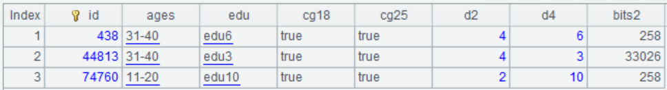
7	=A5.cursor(id,ages,edu,cg18,cg25,d2,d4,bits2).fetch(100)

A1-A4: define and generate pseudo table objects, which can be put into global variables to avoid redefining and generating the object every time;

A5: filter the pseudo table. Now we can utilize the pseudo fields such as the boolean fields cg18 and cg25, as well as the enumeration fields ages and edu. SPL will automatically perform the conversion between pseudo field and real field.

A6: calculate the number of deduplicated customers;

A7: retrieve relevant fields and observe the following result:

Incremental data

Since both the cust_dim and the cust_group will generate full data snapshot every month, we just need to regularly convert the snapshots to composite tables for storage each month.

When calculating customer profile, add the year and month to the name of composite table, and dynamically generate the name of composite table or pseudo table based on the year and month in the given parameter.

Practice effect

Under the hardware condition of 12-core CPU and 64G RAM, it only took 4 seconds to perform 12 customer profile calculations.

Postscript

In the customer profile analysis scenarios, it often needs to perform filter calculation based on the combined conditions of enumerated dimension and binary tag.

When the total amount of data is huge, the operation performance depends primarily on the filtration by combined conditions. Since these conditions are very arbitrary, and we can neither calculate in advance nor count on index, an efficient hard traversal ability is required.

The boolean dimension sequence mechanism and the binary tag bitwise storage mechanism of SPL can effectively solve this problem.