8.1 Foreign key association
8.1.1 Ordinary foreign key association
Part of the data in the sales record table, city information table and product information table are given as below:
Sales record table (fact table):
| recordid | product | product_city | sale_city | amount | … |
|---|---|---|---|---|---|
| sr100001 | p1006 | c105 | c103 | 603 | … |
| sr100002 | p1005 | c105 | c102 | 1230 | … |
| sr100003 | p1003 | c102 | c102 | 885 | … |
| … | … | … | … | … | … |
City information table (dimension table):
| cityid | name | state | … |
|---|---|---|---|
| c101 | New York | New York | … |
| c102 | Miami | Florida | … |
| c103 | Los Angeles | California | … |
| … | … | … | … |
Product information table (dimension table):
| productid | pclass | … |
|---|---|---|
| p1001 | A | … |
| p1002 | A | … |
| p1003 | B | … |
| … | … | … |
Perform the following calculations based on the above data:
1. One fact table and one dimension table - aggregate the sales of each product.
2. One fact table and multiple dimension tables - count the sales of each product of each state.
3. Reuse dimension table
1) Find the sales record of product sold and manufactured in the same state.
2) Calculate the sales of product sold in California.
3) Calculate the total sales of each state as the place of production.
4. Multi-layer dimension table – find the sales records of product manufactured and sold in the same state.
Sometimes, the city information of a certain product is not in the sales record table but in the product information table. In this case, the association is a multi-layer dimension table association.
The modified sales record table and product information table are as follows:
Sales record table 2:
| recordid | product | sale_city | amount | … |
|---|---|---|---|---|
| sr100001 | p1003 | c104 | 380 | … |
| sr100002 | p1005 | c103 | 400 | … |
| sr100003 | p1003 | c104 | 626 | … |
| … | … | … | … | … |
Product information table 2:
| productid | product_city | … |
|---|---|---|
| p1001 | c104 | … |
| p1002 | c103 | … |
| p1003 | c102 | … |
| … | … | … |
SPL
| A | B | |
|---|---|---|
| 1 | =file(“SaleRecord.csv”).import@tc() | |
| 2 | =file(“Product.csv”).import@tc() | |
| 3 | =A1.switch(product,A2:productid) | /1. One fact table and one dimension table |
| 4 | =A3.groups(product.pclass;sum(amount):amount) | /1. One fact table and one dimension table |
| 5 | =file(“City.csv”).import@tc() | |
| 6 | =A1.switch(product,A2:productid;sale_city,A5:cityid) | /2. One fact table and multiple dimension tables |
| 7 | =A6.groups(sale_city.state,product.pclass;sum(amount):amount) | /2. One fact table and multiple dimension tables |
| 8 | =A1.switch(sale_city,A5:cityid;product_city,A5:cityid) | /3. Reuse dimension table |
| 9 | =A8.select(sale_city.state==product_city.state).(recordid) | /3. Reuse dimension table |
| 10 | =A8.select(sale_city.state==“California”).sum(amount) | /The sales of product sold in California |
| 11 | =A8.groups(product_city.state;sum(amount):amount) | /The total sales of each state as the place of production. |
| 12 | =file(“SaleRecord2.csv”).import@tc() | |
| 13 | =file(“Product2.csv”).import@tc() | |
| 14 | =A13.switch(product_city,A5:cityid) | /4. Multi-layer dimension table |
| 15 | =A12.switch(sale_city,A5:cityid;product,A14:productid) | /4. Multi-layer dimension table |
| 16 | =A15.select(sale_city.state==product.product_city.state).(recordid) | /4. Multi-layer dimension table |
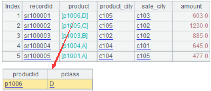
The switch() function is to convert the foreign key field to the corresponding dimension table record. This function only references the dimension table record and does not copy the data and, it can parse multiple association relations at the same time and reuse the relations.
Notes: The above four tasks are independent of each other. Although the codes are written together, when executing, the code for the other three tasks should be commented out to execut expected code, otherwise the field that has been switched cannot be switched again.
The results of A3:

It should be specially noted that the associative relation in SPL is to directly reference the associative record, which allows all associative relations to be established in one go when loading data. In addition, SPL saves the associated results in a pointer manner, making it convenient to use this associative relation for subsequent calculations, which is commonly referred to as pre-association. For example, A8 is the pre-associated data, which can be directly referenced in subsequent A9, A10, and A11.
SQL
1. One fact table and one dimension table - aggregate the sales of each product
SELECT p.pclass AS pclass, SUM(s.amount) AS amount
FROM SaleRecord s
JOIN product p ON s.product = p.productid
GROUP BY p.pclass;
2. One fact table and multiple dimension tables - count the sales of each product of each state
SELECT c.state AS state, p.pclass AS pclass, SUM(s.amount) AS amount
FROM SaleRecord s
JOIN City c ON s.sale_city = c.cityid
JOIN Product p ON s.product = p.productid
GROUP BY c.state, p.pclass;
3. Reuse dimension table 1 - find the sales record of product sold & manufactured in the same state
SELECT s.recordid
FROM SaleRecord s
JOIN City c1 ON s.product_city = c1.cityid
JOIN City c2 ON s.sale_city = c2.cityid
JOIN Product p ON s.product = p.productid
WHERE c1.state = c2.state;
4. Reuse dimension table 2 - calculate the sales of product sold in California
SELECT SUM(amount) AS amount
FROM SaleRecord s
JOIN City c ON s.sale_city=c.cityid
WHERE c.state = 'California';
5. Reuse dimension table 3 - calculate the total sales of each state as the place of production.
SELECT c.state AS state, SUM(s.amount) AS amount
FROM SaleRecord s
JOIN City c ON s.product_city = c.cityid
GROUP BY c.state;
6. Multi-layer dimension table - find the sales records of product manufactured & sold in the same state.
SELECT s.recordid
FROM SaleRecord2 s
JOIN Product2 p ON s.product = p.productid
JOIN city c ON s.sale_city=c.cityid
JOIN city c2 ON p.product_city=c2.cityid
WHERE c.state=c2.state
ORDER BY s.recordid;
Python
record1=pd.read_csv("../SaleRecord.csv")
product1=pd.read_csv("../Product.csv")
r_pt=pd.merge(record1,product1,left_on="product",right_on="productid") #1.One fact table and one dimension table
pclass_sale=r_pt.groupby('pclass',as_index=False).amount.sum()
ct1=pd.read_csv("../City.csv")
r_ct=pd.merge(record1,ct1,left_on="sale_city",right_on="cityid") #2.One fact table and multiple dimension tables
r_ct_pdt=pd.merge(r_ct,product1,left_on="product",right_on="productid") #2.One fact table and multiple dimension tables
ct_pdt_sale=r_ct_pdt.groupby(['state','pclass'],as_index=False).amount.sum()
r_ct2=pd.merge(record1,ct1,left_on="sale_city",right_on="cityid") #3. Reuse dimension table
r_ct_ct=pd.merge(r_ct2,ct1,left_on="product_city",right_on="cityid",suffixes=('_s', '_p')) /#3. Reuse dimension table
r_ct_p_ct= r_ct_ct[r_ct_ct['state_s']==r_ct_ct['state_p']].recordid.values.tolist()
#ThesalesofproductsoldinCalifornia
hlj_sale_amount=r_ct_ct[r_ct_ct['state_s']=="California"].amount.sum()
#Thetotalsalesofeachstateastheplaceofproduction
state_product_amount=r_ct_ct.groupby(['state_p']).amount.sum()
record2=pd.read_csv("../SaleRecord2.csv")
product2=pd.read_csv("../Product2.csv")
pdt_ct=pd.merge(product2,ct1,left_on="product_city",right_on="cityid")
r_pdt_ct=pd.merge(record2,pdt_ct,left_on="product",right_on="productid") #4. Multi-layer dimension table
r_pdt_ct_ct=pd.merge(r_pdt_ct,ct1,left_on="sale_city",right_on="cityid",suffixes=('_s', '_p')) #4. Multi-layer dimension table
r_ct_p_ct2=r_pdt_ct_ct[r_pdt_ct_ct['state_s']==r_pdt_ct_ct['state_p']].recordid.values.tolist()
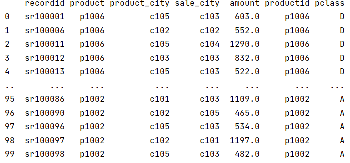
Associating in Python will generate a wide table, which completely copy the data of two tables. For example, the result of r-pt is as follows:

The associative relation created in Python can also be considered as pre-association. For example, the r_ct_ct in the reuse of dimension table can be regarded as the pre-associated result, except that Python creates a large wide table into which all the associative fields are put.
8.1.2 Cycle association
There are two tables: employee information table and department information table:
Employee information table:
| empid | name | dept | state | partner | … |
|---|---|---|---|---|---|
| 1 | FORD | 6 | New York | 12 | … |
| 2 | SCOTT | 2 | Florida | 12 | … |
| 3 | JAMES | 7 | California | 11 | … |
| … | … | … | … | … | … |
Department information table:
| deptid | name | manager | … |
|---|---|---|---|
| 1 | Administration | 20 | … |
| 2 | Finance | 2 | … |
| 3 | HR | 162 | … |
| … | … | … | … |
Perform the following calculations based on the data above:
1. Self-association - list the names of all employees and their partners
2. Cycle association - find the Florida employee of Florida manager
SPL
| A | B | |
|---|---|---|
| 1 | =file(“Employee_1.csv”).import@tc() | |
| 2 | =A1.switch(partner,A1:empid) | /1. Self-association |
| 3 | =A2.new(name,partner.name:name_p) | |
| 4 | =file(“Department2.csv”).import@tc() | |
| 5 | =A4.switch(manager,A1:empid) | |
| 6 | =A1.switch(dept,A5:deptid) | /2. Cycle association |
| 7 | =A6.select(state==“Florida”&&dept.manager.state==“Florida”).(name) | /2. Cycle association |
SQL
1. Self-association - list the names of all employees and their partners
SELECT e.name AS name, p.name AS partner
FROM Employee_1 e
LEFT JOIN Employee_1 p ON e.partner = p.empid;
2. Cycle association - find the Florida employee of Florida manager
SELECT e.name AS employee_name
FROM Employee_1 e
JOIN Department2 d ON e.dept = d.deptid
JOIN Employee_1 m ON d.manager = m.empid
WHERE e.state = 'Florida' AND m.state = 'Florida';
Python
emp=pd.read_csv("../Employee_1.csv")
emp_s=pd.merge(emp,emp,left_on="partner",right_on="empid",suffixes=('', '_p'),how="left")
#1. Self-association
emp_s_name=emp_s[['name','name_p']]
dept2=pd.read_csv("../Department2.csv")
d_emp=pd.merge(dept2,emp,left_on="manager",right_on="empid")
#2. Cycle association
emp_d_emp=pd.merge(emp,d_emp,left_on="dept",right_on="deptid",suffixes=('', '_m'))
#2. Cycle association
Florida_emp_m=emp_d_emp[(emp_d_emp['state']=="Florida") & (emp_d_emp['state_m']=="Florida")].name.tolist()
8.2 Primary key association
Example codes for comparing SPL, SQL, and Python
SPL Official Website 👉 https://www.scudata.com
SPL Feedback and Help 👉 https://www.reddit.com/r/esProcSPL
SPL Learning Material 👉 https://c.scudata.com
SPL Source Code and Package 👉 https://github.com/SPLWare/esProc
Discord 👉 https://discord.gg/2bkGwqTj
Youtube 👉 https://www.youtube.com/@esProc_SPL


