There are generally not many and frequent updates on the target data of OLAP. Usually, the update actions happen when new data is appended or when data is inserted, modified and deleted.

SPL offers the multizone composite table that can effectively shorten the time of handling data updating while ensuring the computing performance.

A multizone composite table is made up of multiple composite table files. We call these composite tables the multizone composite table’s zone tables. Each zone table has its own zone table number.

1. Append-type multizone composite tables

In order to increase performance, SPL needs to store data in order according to certain fields. However, the regularly generated new data cannot always be appended to the existing data in order.

The orders table, for example, stores a large volume of orders data, which consists of customer ids (cid), order dates (odate), order ids (oid), employee ids (eid) and order amounts (amt). It is probably that the orders table will be stored in order according to dimension fields cid and odate in order to enhance performance. Usually, cid field values of the newly-generated orders per day are among the existing customers. The data cannot be directly appended to the historical data, otherwise the order of cid field will be disrupted.

Sorting all data, including the historical data and the new data generated on the current date, or merging them in order each day is time-consuming. SPL’s multizone composite table can address this issue conveniently.

1.1. Storage structure

Take orders table as an example. The multizone composite table consists two zone tables; zone table 1 stores historical data and zone table 2 stores data of the current month. The new data of each day will only be merged with zone table 2 during data appending per day. When zone table 2 continuously absorbs new data through merge for a month, then it will be entirely merged with zone table 1 on the 1^st day of each month.

Remember that zone table numbers must be integers and incremental.

Below is the storage structure of orders table:

1.2. Initialization

During system initiation, a composite table obtains data from the database, the text file or any other data sources. Suppose data of orders table will come from text file orders.txt. Below is the code of creating a new multizone composite table and writing the historical data to it:

	A
1	=file("orders.txt").cursor@t(cid,odate,oid,eid,amt).sortx(cid,odate)
2	=file("orders.ctx":to(2)).create(#cid,#odate,oid,eid,amt;if(month@y(odate)==month@y(now()),2,1))
3	=A2.append@x(A1)

A1 Create cursor on the text file and sort data as needed.

A2 The newly-created multizone composite table is made up of two composite table files. Each file has its number, which is called zone table number. An expression x for computing zone table number is also specified, which is if(month@y(odate)==month@y(now()),2,1).

A3 When append@x is used to append data, SPL computes zone table number expression x on each record to be appended and appends the historical records to zone table 1 and current month data to zone table 2.

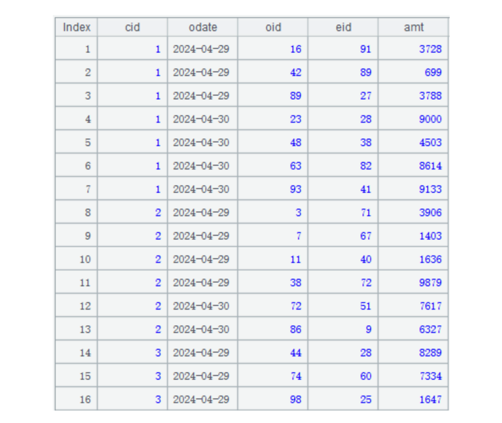
After the multizone composite table is created, data will be stored in its zone tables. For example, data in April stored in the 2^nd zone table (2.orders.ctx) is as follows:

1.3. Implementing the computation

When an append-type multizone composite table is used to perform a computation, the code is almost the same as that where a uni-composite table is used. For example, below is the code of grouping data by customer and computing the transaction amount of the whole year of 2023 for each group:

	A
1	=file("orders.ctx":to(2)).open().cursor(cid,amt;year(odate)==2023)
2	=A1.group(cid;~.sum(amt))

A1 We can select certain zone tables when opening a multizone composite table. Here two zone tables are chosen.

A2 Perform order-based grouping. Both zone table 1 and zone table 2 are ordered by cid; merge them in order and then group records. Though not as fast as the computation performed on a single composite table, this is still fast enough.

1.4. Appending data

Append the daily new orders data generated for orders_new.txt to its zone table 2, and in the 1^st day of each month, merge data of zone table 2 to zone table 1. This way zone table 2 only stores one month of data at most, and it takes not long to perform the daily merge operation. It is also acceptable that it takes a little longer to complete the monthly whole-table merge.

The code is generally like this:

	A	B
1	=file("orders_new.txt").cursor@t(cid,odate,oid,eid,amt).sortx(cid,odate)
2	=file("orders.ctx":to(2))
3	if day(now())==1	=A2.reset@y(A2,if(month@y(odate)==month@y(now()),2,1);A1)
4	else	=file("orders.ctx":2).open()
5		=B4.append@m(A1)
6		>B4.close()

A1 Sort the newly-generated data on the current date by dimension fields.

A3 Check whether the current date is the first day of the month and if it is, B3 merges zone table 1 and zone table 2 as well as the newly-generated data into the multizone composite table orders. After the merge, zone table 1 stores data of the previous months and zone table 2 stores data of the first date in the current month.

A3 Check whether the current date is the first day of the month and if it isn’t, B4, B5 and B6 merges the newly-generated data into zone table 2 in order.

The code of performing the computation using multizone composite table orders is the same.

2. Append-type multizone composite tables – with multizone and multitable

The append-type multizone composite table previously illustrated consists of two zone tables. It is suitable for storing data of medium-size volume. When there is an extremely huge volume of data, we can store them in multiple zones and tables. This can not only increase data appending performance, but quickly delete useless historical data in batches.

2.1. Storage structure

Still take an orders table as the example. We store the historical data in multiple zone tables; each zone table stores data of one month, and uses year/month (yyyyMM) as the zone table number, such as 202402, … and 202405, which store data from February 2024 to May 2024.

The multizone, multitable storage structure is shown in the following figure. In order to distinguish from the previous orders table, this multizone, multitable orders table is named ordersN.

Besides, we use global variables beginMonth and endMonth to represent the starting month 202402 and the ending month 202405 of the orders data.

We can see from this example that zone numbers do not necessarily start from 1. They only need to be incremental.

2.2. Initialization

Suppose data of ordersN comes from text file orders.txt, we create a multizone composite table and write the historical data to it during system initiation. the code of doing this is as follows:

	A	B
1	>env(beginMonth,202403),env(endMonth,202405)
2	=file("orders.txt").cursor@t(cid,odate,oid,eid,amt).sortx(cid,odate)
3	=file("ordersN.ctx":to(beginMonth,endMonth)).create@y(#cid,#odate,oid,eid,amt;month@y(odate))
4	=A3.append@x(A2)	>A3.close()

A1 Specify the beginning month and the ending month. We can take the two values as initialization parameters to pass them in, or use them to find the maximum value and the minimum value of the odate field’s year/month in the historical data. Generally, endMonth is the current month during the initialization.

A2 Sort the original data by cid and odate.

A3 Create a multizone composite table, for which zone table numbers are from beginMonth to endMonth and zone table expression computes the odate’s year/month values.

A4 Write the sorted original orders data to different zone tables of the multizone composite table according to result of computing the zone table expression.

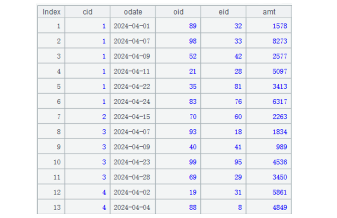
Below is data in zone table 202404:

2.3. Implementing the computation

The code of using an append-type multizone composite table to perform a computation is almost the same as that where a uni-composite table is used. For example, the code for grouping records by customer and computing the total transaction amount in the year 2024 in each group is generally like this:

	A
1	=file("orders.ctx":to(beginMonth,endMonth)).open().cursor(cid,amt;year(odate)==2024)
2	=A1.group(cid;~.sum(amt))

A1 We can select certain zone tables when opening a multizone composite table. Here all zone tables are chosen.

A2 Perform order-based grouping. Each zone table is ordered by cid; merge the multiple files meeting the specified date condition in order and then group records. Though not as fast as the computation performed on a single composite table, the speed is still satisfactory.

For cases where batches of outdated data are removed, just don’t let the zone tables containing the outdated data participate in the computation. For example, if data of February is outdated, just change value of beginMonth from 2 to 3.

Actually, it is not necessarily that zone table numbers in a multizone composite table are continuous. For example, we need to compute data in March and May and can write A1 as =file(“orders.ctx”:[3,5]).open().cursor(cid,amt). We only need to keep the zone table numbers incremental. That is to say, sometimes the newly-generated multizone composite table and the one used for the computation are not made up of the same zone tables. We can select certain zone tables as needed to perform the computation.

But, we should first check whether beginMonth<=3 && 5<=endMonth are true.

2.4. Appending data

Append the daily new orders data generated for orders_new.txt to the last zone table. And on the 1^st day of each month, create a new zone table and merge the newly-generated data to the new zone table. This can avoid the merge of newly-generated data with a huge volume of historical data.

The code is generally like this:

	A	B
1	=file("orders_new.txt").cursor@t(cid,odate,oid,eid,amt).sortx(cid,odate)
2	if day(now())==1	>endMonth=month@y(now())
3		=file("ordersN.ctx":[beginMonth]).open()
4		=B3.create@y(file("ordersN.ctx":[endMonth]))
5		=B4.append@i(A1)
6		>B3.close(),B4.close()
7	else	=file("ordersN.ctx":endMonth).open()
8		=B7.append@m(A1)
9		>B7.close()

A1 Sort the newly-generated data by cid and odate.

A2 Check whether the date is the first day of the current month and if it is, execute code in B2~B6.

B2 Change the ending month to the current month.

B4 Create a new zone table for the current month, and add the newly-generated data to this zone table.

A2 Check whether the date is the first day of the current month and if it isn’t, execute code in B7~B9.

B7 Open the ending month zone table.

B8 Merge the newly-generated data to the ending month in order.

The code after data is appended is the same as that in the above.

3. Update-type multizone composite tables

An append-type multizone composite table cannot be used to handle updates (insert, delete and modify) on the historical data.

When only a small amount of data is updated, we can use the uni-composite table’s patch zone to handle the update. Find detailed explanation in Performance Optimization - 2.6 [Dataset in external storage] Data update and multi-zone composite table.

When a large volume of data is involved in the update and the patch zone probably cannot hold the updated data, we need the update-type multizone composite table to do this job. An update-type multizone composite table must have a primary key.

Let’s first look at a scenario only involving insert and modification and without the delete.

3.1. Storage structure

An update-type multizone composite table can store the historical data in one zone table and the newly-generated data in the other zone table.

Suppose we store the historical data in zone table 1 and the newly-generated data in the current month in zone table 2, we get an update-type orders table having the following structure and name it ordersModify in order to differentiate it from the previous append-type orders table.

When performing the daily data updating, merge the newly-generated data only with zone table 2. On the first day of every month, perform the full merge between zone table 2 and zone table 1.

3.2. Initialization

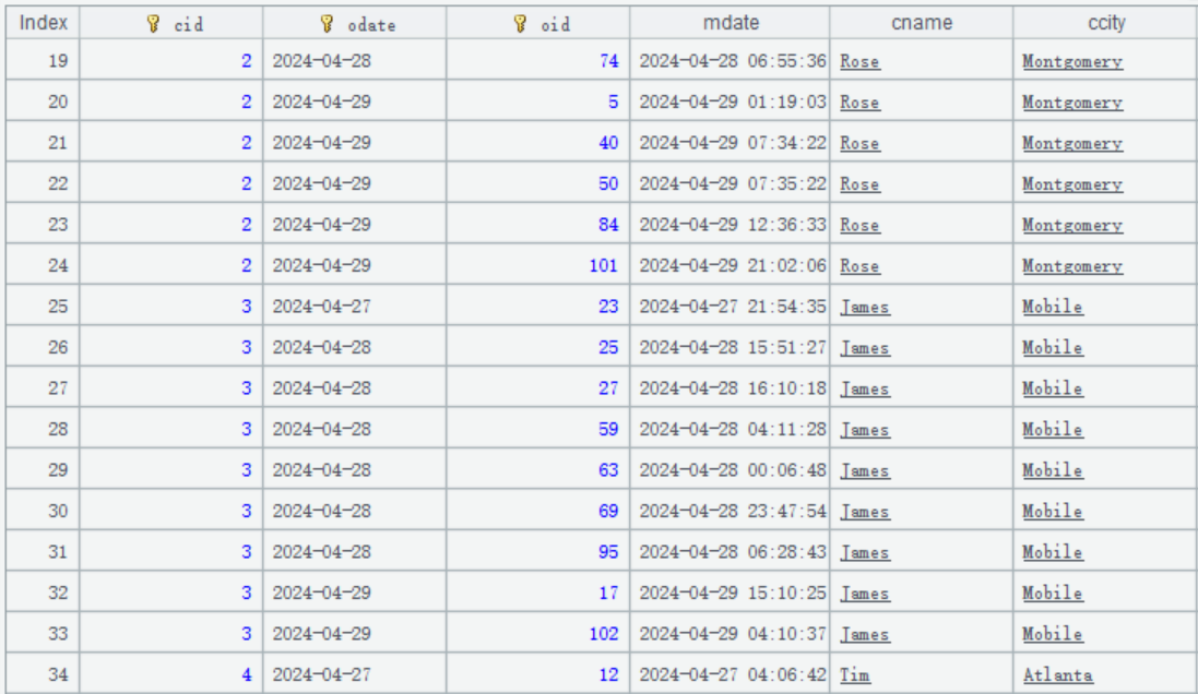
Let’s look at how to write code for initialization. The orders table has a primary key consisting of cid (customer id), odate (order date) and oid (order id). The customer names (cname) and cities that customers are based (ccity) are also redundant to the orders table.

Also, remember to add a record modification time field mdate. Now here is the orders data:

To initialize the system, first we write the historical data to zone table 1. Here’s the code:

	A	B
1	=file("orders.txt").cursor@t(cid,odate,oid,cname,ccity,eid,amt).sortx(cid,odate,oid)
2	=file("ordersModify.ctx":[1]).create@y(#cid,#odate,#oid,cname,ccity,eid,amt;1)
3	=A2.append@i(A1)	>A3.close()

A2 creates zone table 1. A3 writes the historical data to zone table 1.

3.3. Data updating – without deletion

Suppose the to-be-updated data coming from the source data is stored in orders_new.txt. Below is the to-be-updated data on April 30 2024:

The to-be-updated data is usually ordered by the update time, and it is likely that a record having the same primary key will modify data multiple times.

In the above table, the record whose index is 5 will modify the orders record whose primary key is [2, 2024-04-29, 101] by changing ccity to San Francisco; and the record whose index is 11 modifies ccity of the same orders record to Atlanta.

On May 1 2024, the to-be-updated data is as follows:

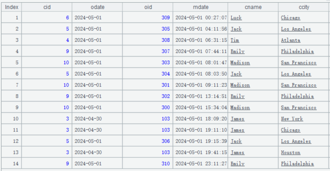
First, the record whose index is 10 insert an orders record whose primary key is [3, 2024-05-01, 103]. Then the records whose indexes are respectively 11 and 13 modify the orders record twice to change ccity to Chicago and Houston.

Below is the code of updating data of ordersModify:

	A	B
1	=file("orders_new.txt").cursor@t(cid,odate,oid,eid,amt).sortx(cid,odate,oid,mdate)
2	if day(now())==1	=file("ordersModify.ctx":[1,2]).reset@wy(file("ordersModifyNew.ctx":[1]))
3		=movefile@y("1.ordersModifyNew.ctx","1.ordersModify.ctx")
4		=file("ordersModify.ctx":1).open()
5		=B5.create@y(file("ordersModify.ctx":[2]))
6		>B6.close(),B5.close()
7	=file("ordersModify.ctx":[2]).reset@wy(;A1)

A1 The to-be-updated data coming from the source data. Note: It is a must that the to-be-updated data is ordered by the primary key and the update time in ascending order.

A2 Check whether the current date is the first day of the current month and if it is, execute code in B2~B6; otherwise, jump to A7.

B2 Merge zone table 1 and zone table 2 to the new multizone composite table ordersModifyNew.ctx’s zone table 1. The @w option used in reset() function automatically handles records having same primary key in zone table 1 and zone table 2 by retaining the one with the largest mdate value.

B3 Rename the new multizone composite table’s zone table 1 to overwrite the original zone table 1.

B4~B6 Clear the existing data and create a new zone table 2.

A7 Merge the to-be-updated data table cursor to zone table 2. The @w option used in reset() function automatically handles records having same primary key in zone table 2 and the to-be-updated data table cursor by retaining the one with the largest mdate value.

3.4. Implementing the computation

The code of querying and computing data in ordersModify is generally like this:

	A	B
1	=file("ordersModify.ctx":[1,2]).open().cursor@wx().fetch(100)
2	=file("ordersModify.ctx":[1,2]).open().cursor@wx()
3	=A2.group(cid;~.cname,~.sum(amt))

A1 queries zone table 1 and zone table 2 in ordersModify. The @w option used in cursor() function handles records with same primary key by retaining the one in zone table 2.

After data updating on May 1, A1 gets the following result:

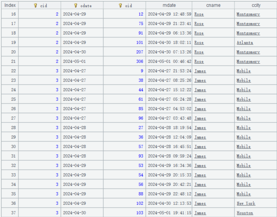
In the orders record whose primary key is [2, 2024-04-29, 101], ccity field is changed to Atlanta.

In the orders record whose primary key is [3, 2024-04-29, 102], ccity field is changed to New York.

An orders record whose primary key is [3, 2024-05-01, 103] is inserted to the target position and its ccity field is changed to Houston.

A3 performs an order-based grouping & aggregation operation according to cid.

3.5. Data updating including deletion

Add deletion mark field

To handle data deletion, we need to add a deletion mark field to the update-type multizone composite table. The deletion mark field is the first field after the dimension field(s); a true value represents to-be-deleted, a false value represents to-be-modified and a null value means to-be-inserted.

For example, the orders table becomes like this after deletion mark field mflag is added:

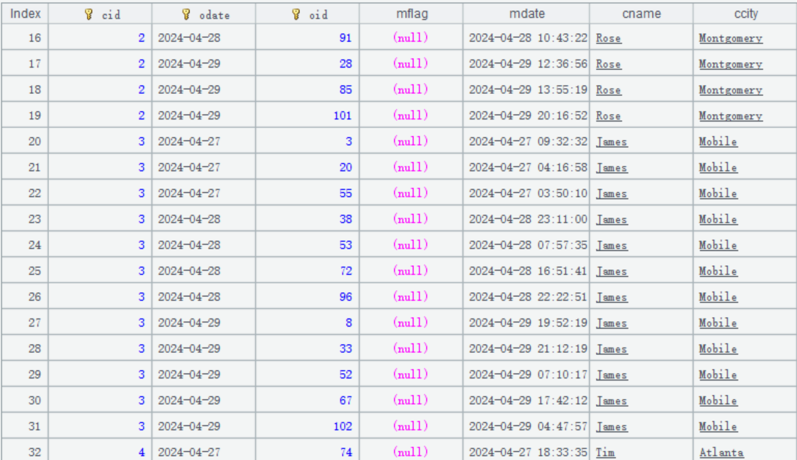
System initiation

Here the code is a little different from that of merging the historical data to zone table 1 when no deletion occurs at system initiation:

	A	B
1	=file("orders.txt").cursor@t(cid,odate,oid,mflag,mdate,cname,ccity,eid,amt).sortx(cid,odate,oid)
2	=file("ordersModify.ctx":[1]).create@dy(#cid,#odate,#oid,mflag,mdate,cname,ccity,eid,amt;1)
3	=A2.append@i(A1)	>A3.close()

A2 creates zone table 1. The @d option working with create() function means the first field mflag after the primary key is the deletion mark. SPL will automatically insert, delete and modify data during data merging.

The daily to-be-updated orders data table orders_new.txt coming from the source data also needs to have a deletion mark field mflag. For example, the to-be-updated data on April 30 is like this:

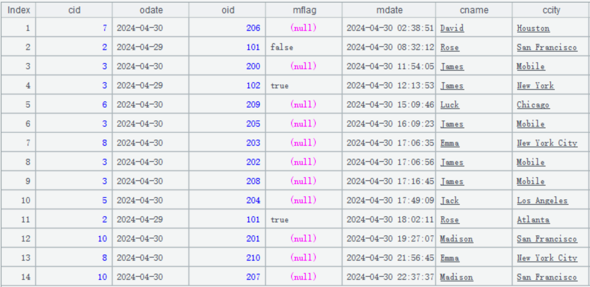
The to-be-updated data is ordered by modification time mdate. There are also records having same primary key, for example:

The record whose index is 2 will modify the orders records whose primary key is [2, 2024-04-29, 101].

The record whose index is 4 will delete the orders records whose primary key is [3, 2024-04-29, 102].

The record whose index is 11 will delete the orders records whose primary key is [2, 2024-04-29, 101].

All the other modifications are appending actions.

Updating data and implementing the computation

The code is the same as that for cases where no deletions occur.

Three statuses of deletion mark

As we mentioned above, the deletion actions have three statuses. But why do we use false and null to distinguish modification from insertion? Let’s take the to-be-updated data on April 30 to illustrate the reason.

As this date isn’t the first day of the current month, we only need to merge the to-be-updated data to zone table 2. As the update without deletion, we also need reset@w() function to automatically handle the merging.

In the above table, the record whose index is 11 has the primary key [2, 2024-04-29, 101] and deletion mark true meaning that the orders record having this primary key will be deleted.

Since zone table 1 does not participate in the computation, reset@w cannot know whether there is a record having the same primary key in it. In this case, we should find the to-be-updated record having the same primary and whose mdate value is earlier and determine how to handle the deletion according to it:

1. In the above table, the earlier to-be-updated table record whose index is 2 also has the primary key [2, 2024-04-29, 101] but its deletion mark is false that means to-be-modified. This implies that there is a record having the same primary key in zone table 1. Therefore, this record marked as to-be-deleted should be retained and the previous modification action will be discarded.

2. If there is a to-be-updated table record having the primary key [2, 2024-04-29, 101] and with the deletion mark null meaning to-be-inserted before this update record. This allows us to infer that there isn’t a record having this primary key in zone table 1. And both this update record marked as deleted and the one marked as inserted should be discarded.

3. Suppose there isn’t an update record having primary key [2, 2024-04-29, 101] before the current one. We can infer that there is a record having such a primary key in zone table 1, so this record marked as to-be-deleted should be retained.

According to this example, the deletion mark must have three statuses: true, false and null; otherwise reset@w cannot automatically handle update cases involving delete actions.

4. Update-type multizone composite tables – with multizone and multitable

In some scenarios, there is an extremely huge volume of historical data and the updates are frequent.

We can use the multizone and multitable method to handle such an updating case. For example, each daily update generates a new zone table and those zone tables will be merged and rearranged at the right time.

4.1. Storage structure

If we create a new zone table for each day’s newly-generated data, the multizone, multitable storage structure is as follows:

Put the historical data in zone table 1.

Store the updated data on April 30 in the newly-created zone table 20240430, and that on May 1 and May 2 respectively in zone tables with corresponding date names.

4.2. Initialization

Let’s look at how to write the initialization code. The orders data is generally like this:

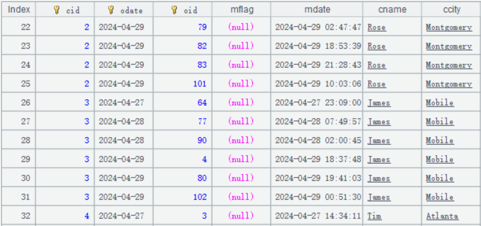
First, merge the historical data with zone table 1 at system initialization. The code of doing this is like this:

	A	B
1	=file("orders.txt").cursor@t(cid,odate,oid,mflag,mdate,cname,ccity,eid,amt).sortx(cid,odate,oid)
2	=file("ordersModify.ctx":[1]).create@dy(#cid,#odate,#oid,mflag,mdate,cname,ccity,eid,amt;1)
3	=A2.append@i(A1)	>A3.close()

A2 creates zone table 1. Here create() function works with @d option; if no deletion actions are involved, the option can be absent.

A3 Append the historical data to zone table 1.

4.3. Data updating

We still use reset@w() function to handle the updates on a multi-zone table composite table. For example, here is the code of updating data on May 2 2024:

	A
1	=int(string(now(),"yyyyMMdd"))
2	=file("orders_new.txt").cursor@t().sortx(cid,odate,oid,mdate)
3	=file("ordersModify.ctx":1).open()
4	=A3.create@y(file("ordersModify.ctx":[A1]))
5	>A4.close(),A3.close()
6	=file("ordersModify.ctx":[A1]).reset@wy(;A2)

A1 gets zone table number 20240502. A2 sorts the to-be-updated data by primary key and update time (mdate).

A3 ~ A5 creates a new zone table 20240502 using zone table 1. A6 merges the to-be-updated data with zone table 20240502.

4.4. Merging zone tables and implementing the computation

There are more and more zone tables as time goes by. We need to merge them at a suitable time. There are two types of merging:

Type 1: Full merge

Merge all the other zone tables to zone table 1, as shown by the following figure:

Below is the code of performing the full merge:

	A
1	=file("ordersModify.ctx":[1,20240430,20240501,20240501]).reset@wy(file("ordersModifyNew.ctx":[1]))
2	=movefile@y("1.ordersModifyNew.ctx","1.ordersModify.ctx")

A1 merges all zone tables as a new multizone composite table. A2 overwrites zone table 1 of the original multizone composite table with zone table 1 of the new multizone composite table.

Below is the code of implementing the computation after all zone tables are merged:

	A
1	=file("ordersModify.ctx":[1]).open().cursor@x().fetch(100)
2	=file("ordersModify.ctx":[1]).open().cursor@x()
	=A2.group(cid;~.cname,~.sum(amt))

Type 2: Partial merge

Choosing a number of updated zone tables to merge them can also reduce the number of zone tables. For example, we merge zone table 20240430 and zone table 20240501 into a new zone table 2, as shown in the following figure:

Or we can merge 20240501 and 20240502 as a new 20240502. Just make sure the zone table numbers are incremental.

Below is the code of performing the partial merge:

	A
1	=file("ordersModify.ctx":[20240430,20240501]).reset@wy(file("ordersModifyNew.ctx":[2]))
2	=movefile@y("2.ordersModifyNew.ctx","2.ordersModify.ctx")

A1 merges the selected zone tables as a new multizone composite table. A2 overwrites zone table 2 of the original multizone composite table with zone table 2 of the new multizone composite table.

Below is the code of implementing the computation after certain zone tables are merged:

	A
1	=file("ordersModify.ctx":[1,2,20240502]).open().cursor@x().fetch(100)
2	=file("ordersModify.ctx":[1,2,20240502]).open().cursor@x()
	=A2.group(cid;~.cname,~.sum(amt))

Note: Numbers of all currently valid zone tables should be included when we implement the computation. For example, if we just write [1, 20240502] in A1, the updates of zone table 2 will be left out and result will be wrong.

This is different from the case of append-type multizone composite table. A multizone, multitable append-type composite table allows selecting zone table numbers as needed and they can be discontinuous. For example, the filtering condition specifies March and May, then zone table of April can be skipped.

5. Composite table application routines

This essay mainly focuses on the principles and basic applications of multizone composite tables. Both the data appending and updating we’ve previously explained are executed during each break of the business computations, such as the time after each day’s work. We call this kind of appending and updating the cold mode.

In actual practices, we can also support the hot mode based on the multizone composite table. This means that we can perform business computations while appending and updating data.

The specific operations are a little complicated. See Data Maintenance Routine for detailed explanations.